Bubble sort - Insertion sort

Introduction

Overview

This post will cover two sorting algorithms - bubble sort and insertion sort. They are simple, yet they perform poorly in real world as the number of elements needed to be sorted gets larger. Therefore, they are often used as educational tools for introductory courses to algorithms, and more importantly, as typical examples of inefficient algorithms.

The sorting problem

The problem called sorting problem is specified by the following input and output pair:

• Input: A sequence of $n$ numbers $(a_1, a_2, …, a_n)$.
• Output: A permutation $(b_1, b_2, …, b_n)$ of the input sequence such that $ b_1 \le b_2 \le … \le b_n $.

A sequence $(a_n)$ is sorted if and only if for all $i \lt j, a_i \le a_j$.

Why is sorting necessary?

There are several obvious applications of sorting such as organizing posts by date or maintaining a telephone directory in alphabetical order. Besides that, some problems will become easier thanks to sorting, for example binary search, finding a median, and identifying statistical outliers.

Bubble sort

What is Bubble sort?

Bubble sort is a comparison sort that works by repeatedly stepping through the list, comparing each pair of adjacent items and swapping them if they are in the wrong order. If we have $n$ items, we need to iterate over the list for $n-1$ times. The algorithm is known as bubble sort because after every complete iteration, the largest element in the given array bubbles up towards the last place, just like the movement of air bubbles in the water that float to the surface and stay there.

Walk-through example

Consider we need to sort the array [6, 2, 5, 3, 9] in ascending order. In each step, elements that are being compared are written in bold.

First pass

• [6, 2, 5, 3, 9] $ \rightarrow $ [2, 6, 5, 3, 9], The algorithm compares 6 and 2, and swaps them because 6 > 2
• [2, 6, 5, 3, 9] $ \rightarrow $ [2, 5, 6, 3, 9], Swap since 6 > 5
• [2, 5, 6, 3, 9] $ \rightarrow $ [2, 5, 3, 6, 9],
• [2, 5, 3, 6, 9] $ \rightarrow $ [2, 5, 3, 6, 9], No swap because these elements are in correct order (6 < 9)

Second pass

• [2, 5, 3, 6, 9] $ \rightarrow $ [2, 5, 3, 6, 9]
• [2, 5, 3, 6, 9] $ \rightarrow $ [2, 3, 5, 6, 9], Swap because 3 < 5
• [2, 3, 5, 6, 9] $ \rightarrow $ [2, 3, 5, 6, 9], No swap because these elements are in order
• [2, 3, 5, 6, 9] $ \rightarrow $ [2, 3, 5, 6, 9],

Third pass

• [2, 3, 5, 6, 9] $ \rightarrow $ [2, 3, 5, 6, 9]
• [2, 3, 5, 6, 9] $ \rightarrow $ [2, 3, 5, 6, 9]
• [2, 3, 5, 6, 9] $ \rightarrow $ [2, 3, 5, 6, 9]
• [2, 3, 5, 6, 9] $ \rightarrow $ [2, 3, 5, 6, 9]

The array is already sorted after the second pass, but the algorithm does not know whether it is completed. In this case, as we specify four passes for the array of five elements, the algorithm needs two more passes to complete without changing anything in the array.

The redundant passes through the list motivate us to think about how to eliminate them. In fact, we can optimize this algorithm by adding an extra variable swapped inside a loop. If there occurs swapping of elements, swapped will be set to true. Otherwise, it is set to false.

Implementation

Python code for Bubble Sort algorithm

def bubble_sort(arr):
    n = len(arr)
    for i in range(0, n - 1):
        for j in range(0, n - i - 1): #Last i elements are already in place
            if arr[j] > arr[j+1]:
                arr[j], arr[j+1] = arr[j+1], arr[j]

Optimized Bubble Sort

def bubble_sort(arr):
    n = len(arr)
    for i in range(0, n - 1):
        swapped = False
        for j in range(0, n - i - 1): #Last i elements are already in place
            if arr[j] > arr[j+1]:
                arr[j], arr[j+1] = arr[j+1], arr[j]
                swapped = True
        if swapped == False:
            return

Complexity Analysis

1. Time complexity

To determine time complexity, we need to count the number of comparisons, which dominates the number of swaps (the algorithm always compare two adjacent elements but doesn’t necessarily swap them).

Pass	Number of comparisons
1st	n - 1
2nd	n - 2
3rd	n - 3
…	…..
last	1

Therefore, the total number of comparisons is \((n-1) + (n-2) + (n-3) + ... + 1 = \frac{n(n-1)}{2} = O(n^2)\)

Standard bubble sort

• Worst case and average case: In both cases, the algorithm needs to do $N$ iterations. In each iteration, it does the same number of comparisons, although there are fewer swaps in average case compared to worst case. Therefore, the time complexity for both cases: $ O(n^2) $

• Best case (the array is already sorted): The time complexity of standard algorithm is still $ O(n^2) $ because the the algorithm does not know if the array is in correct order.

Optimized bubble sort

• Worst case and average case: Though there is a little improvement in the performance of optimized version in the worst and average case, its time complexity is still $ O(n^2) $.
• Best case: Since the array is already sorted, the algorithm traverse over it once and terminate after finding no possible swaps. Hence, the time complexity is $ O(n) $.

2. Space complexity

Because bubble sort is a in-place sorting algorithm, the auxiliary space for it is $ O(1) $.

Insertion sort

How does Insertion sort work?

The algorithm works like most people would sort playing cards in their hands. We start with a section of card we have sorted, then we add or “insert” one more card into its proper place in that sorted section. Eventually, after all of the cards are inserted into their place one after another, we’ll have the entire hand of cards sorted.

Algorithm

To sort an array of $n$ elements in ascending order:

1. Iterate the array from the second element.
2. At each iteration, pick the current element as a key and compare it with elements before it.
3. If the key element is smaller than the element before it, shift that element to the right to create space for the key. The process is repeated until the key is inserted into correct position.
4. After all iterations, we should get our array sorted in ascending order.

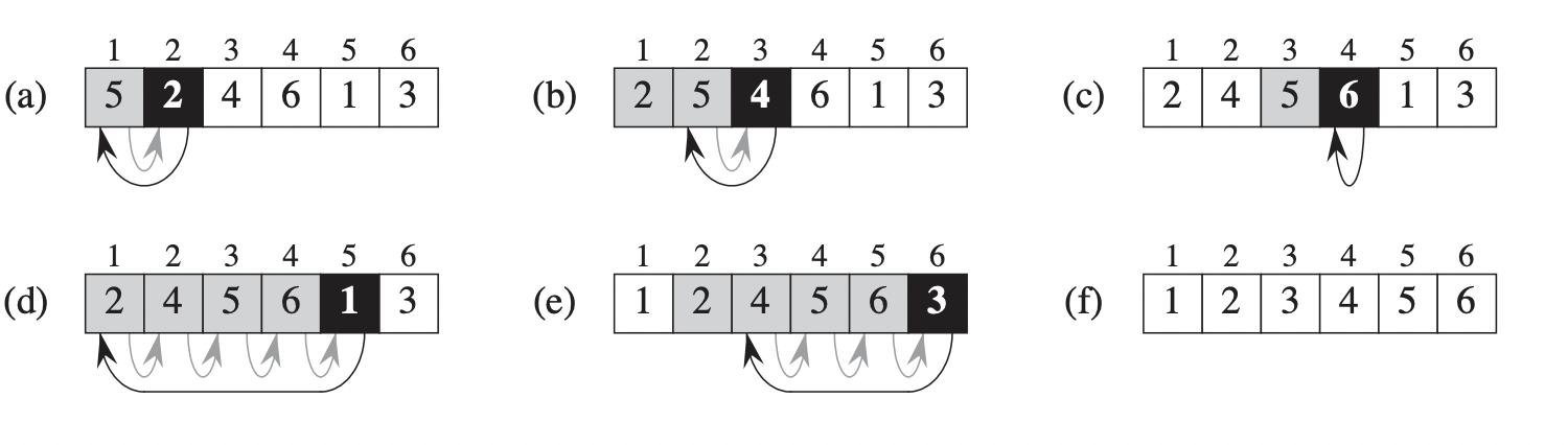Example of Insertion Sort 1

Binary Insertion sort

When the algorithm first starts, the first element by itself is already sorted. Therefore, after $k$ iterations, there are $k+1$ elements that are in correct order. Knowing that property, we can use binary search in $A[0…i-1]$ to find right position the for key $A[i]$ instead of scanning through all the elements before it. ($A[i]$ is the element at index $i$ of array $A$)

We know that binary search algorithm runs in $O(log_2n)$ for an input of size $n$. Using binary search, we can reduce the time for searching position for the key, but shifting elements to the right to insert key still takes $\Theta(n)$ time.²

Implementation

def insertion_sort(arr):
    n = len(arr)
    for i in range(1, n):
        key = arr[i]
        j = i - 1
        while j > -1 and arr[j] > key:
            arr[j+1] = arr[j]   #Shift elements that are greater than key to the right
            j -= 1              
        arr[j+1] = key          #Insert key to the right position

Complexity analysis

1. Time complexity

To calculate the running time of insertion sort, we need to know the amount of time required to execute each line of the algorithm. We assume that the $i$th line takes $c_i$ time to run, where $c_i$ is a constant. For each $j=2,…,n$, where $n$ is the number of elements in array $A$, we let $t_j$ denote the number of times the while loop in line $4$ is executed for that value of $j$ (we use one-based indexing in this example). It is important to note that the test in while or for loop runs one more time than the body of loop because it needs to check the condition. If it fails, the loop will terminate.¹

insertion_sort(A):           cost    times

1  for $j=2$ to $n$:           $c_1$                    $n$

2    $key = A[j]$                                      $c_2$                    $n-1$

3    $i = j - 1$                                         $c_3$                    $n-1$

4    while $i > 0$ and $A[i] > key:$       $c_4$                    $\sum_{j=2}^n t_j$

5      $A[i+1] = A[i]$                      $c_5$                    $\sum_{j=2}^n(t_j-1)$

6      $i = i - 1$                                  $c_6$                    $\sum_{j=2}^n(t_j-1)$

7    $A[i+1] = key$                               $c_7$                    $n-1$

The running time of the algorithm is the sum of the running time of each statement. A statement that runs in $c_i$ time and executes $n$ times will takes $c_{i}n$ time to run in total. Thus, the running time $T(n)$ of insertion_sort(A) is

\[T(n) = c_1n + c_2(n-1) + c_3(n-1) + c_4\sum_{j=2}^n t_j + c_5\sum_{j=2}^n(t_j-1) \\ + c_6\sum_{j=2}^n(t_j-1) + c_7(n-1)\]

In addition to the size of input, the algorithm’s running time may depend on which input of that size is given.

• Firstly, we consider the best case, which is the array is already sorted. This means that for each $j=2,3,…,n$, $A[i] \le key$  with $i = j-1$. The inner loop only checks condition but doesn’t run the loop body. Therefore, $t_j = 1$ for $j=2,3,…,n$, and the best-case running time is

\[T(n) = c_1n + c_2(n-1) + c_3(n-1) + c_4\sum_{j=2}^n 1 + c_7(n-1) \;\;\;\;\;\;\\ \;\;\;\;\,= c_1n + c_2(n-1) + c_3(n-1) + c_4(n-1) + c_7(n-1) \\ = (c_1 + c_2 + c_3 + c_4 + c_7)n - (c_2+c_3+c_4+c_7) \;\;\;\,\\ = O(n) \qquad\qquad\qquad\qquad\qquad\qquad\qquad\qquad\qquad\;\]

• Next, we consider the worst case - the array is sorted in descending order. The algorithm must compare each element $A[j]$ with each element in the subarray $A[1…j-1]$, so $t_j=j$ for $j=2,3,…,n$. Notice that

\[\sum_{j=2}^n j = \frac{(n+2)(n-1)}{2} = \frac{n^2+n-2}{2} = \frac{n(n+1)}{2} - 1 \;\\ \sum_{j=2}^n (j-1) = \frac{n(n-1)}{2} \qquad\qquad\qquad\qquad\qquad\qquad\qquad\]

Thus, the running time of Insertion sort in worst case is

\[T(n) = c_1n + c_2(n-1) + c_3(n-1) + c_4(\frac{n(n+1)}{2} - 1) \qquad\qquad\qquad\;\;\;\\ + c_5(\frac{n(n-1)}{2}) + c_6(\frac{n(n-1)}{2}) + c_7(n-1) \qquad\qquad\qquad\\ = (\frac{c_4}{2} + \frac{c_5}{2} + \frac{c_6}{2})n^2 + (c_1 + c_2 + c_3 + \frac{c_4}{2} - \frac{c_5}{2} - \frac{c_6}{2} + c_7)n \\ - (c_2 + c_3 + c_4 + c_7) \qquad\qquad\qquad\qquad\qquad\qquad\qquad\qquad\\ = O(n^2) \qquad\qquad\qquad\qquad\qquad\qquad\qquad\qquad\qquad\qquad\qquad\;\;\]

When calculating the asymptotic running time of an algorithm, we consider only the leading term of a formula and ignore the lower-order terms and constant factors because they are less significant as inputs become larger. This observation will allow us to determine the efficiency of a complex algorithm in a more simple way.

2. Space complexity

Insertion sort is an in-place sorting algorithm. Thus, its space complexity is $O(1)$.

Conclusion

In this post, we covered two simple but inefficient sorting algorithms. Due to their inefficiency, these two algorithms are not used widely in practice. Later posts will cover more advanced sorting algorithms which have better asymptotic running times.

References

1. Thomas H. Cormen, Charles E. Leiserson, Ronald L. Rivest, Clifford Stein: Introduction to Algorithms, 3rd Edition. MIT Press 2009, ISBN 978-0-262-03384-8, pp. 17-29. ↩ ↩²

2. Srini Devadas, S. 6.006 Introduction to Algorithms: Lecture 3, Fall 2011. ↩