Heaps - Heapsort
Introduction
In this post, we will discuss a new sorting algorithm that works based on an abstract data type (ADT): a heap, and so we call this algorithm heapsort. The running time of heapsort is $O(n \lg n)$, which is asymptotically faster than bubble sort and insertion sort. Although heapsort has the same time complexity as mergesort, the main advantage of heapsort over mergesort is sorting in place.
In previous posts, we have seen how quicksort and mergesort work based on the divide-and-conquer paradigm. This post will introduce a new algorithm design technique: using data structures to store and manipulate data.
Overview
We will start by briefly discussing the properties of heaps and basic operations on this data structure. Then, we explore the main procedures of the heapsort algorithm. Following that, we analyze the time complexity of these procedures and the heapsort algorithm. In addition, we will prove the properties of binary trees (heaps), which are essential to computing the running time of basic operations on the heap data structure.
Heaps
Definition
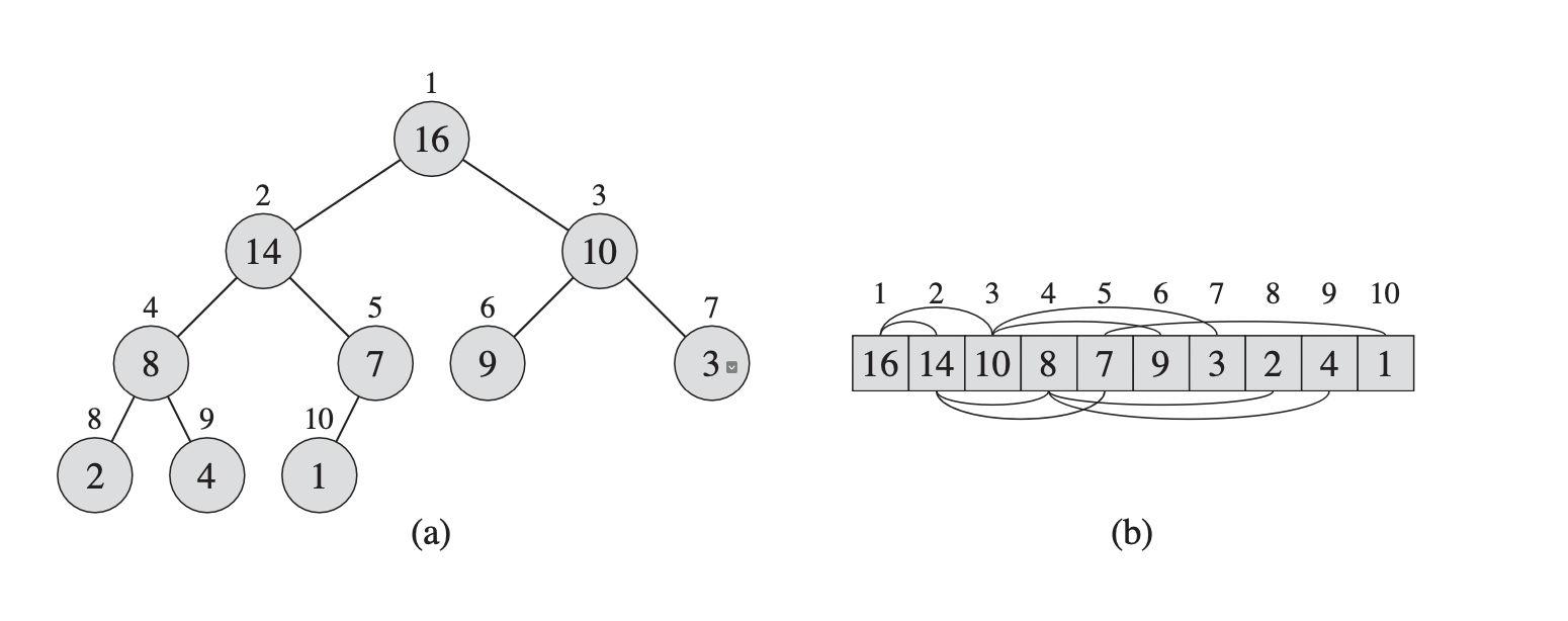
A binary heap is often constructed as a nearly complete binary tree from an array object where each node of the binary tree represents an element of the array. We build the heap by placing each element in the array into a binary tree from left to right, level by level. By constructing the tree in this way, we can ensure that it is filled up all levels except possibly the lowest. The tree with this layout is called a nearly complete binary tree, which is shown below.
 |
|---|
| A heap built from an array 1 |
An array $A$ representing a heap is an object with two attributes: $A.length$, which returns the number of elements in the array $A$, and $A.heap\mathrm{-}size$, which gives the number of elements of the heap stored in the array $A$. Elements in the array $A$ are not always in the heap, so $0 \le A.heap\mathrm{-}size \le A.length$. If we use one-based indexing, the root of the tree (the heap) is $A[1]$. Also, knowing the index $i$ of a node, we can easily compute the indices of its parent, left child, and right child:
\[\begin{align} \mathrm{parent}(i) &= \left\lfloor\frac{i}{2}\right\rfloor \\ \mathrm{leftChild}(i) &= 2i \\ \mathrm{rightChild}(i) &= 2i + 1 \\ \end{align}\]These operations should take constant time to compute.
Max-heaps and Min-heaps
There are two types of binary heaps: max-heaps and min-heaps. Each kind of heaps has a specific heap property that every node of the heaps needs to satisfy. In a max-heap, every node, except the root node, has a value smaller than the value of its parent. Hence, the largest element in a max-heap is always stored at the root.
Max-heap property: $A[\mathrm{parent}(i)] \ge A[i]$
We define a min-heap in a similar way, where every node $i$ of it other than the root node satisfies:
Min-heap property: $A[\mathrm{parent}(i)] \le A[i]$
Based on this property, the smallest element of a min-heap is at the root of the binary heap.
In this post, we will use max-heaps for the heapsort algorithm. Viewing a heap as a tree, we define the height of a node in a heap to be the number of edges on the longest simple path from the node to a leaf and the height of the heap to be the height of its root. We can also define the depth of a node as the length of the path from the heap root to that node. Hence, the height of a heap is equal to its depth. We can see that the number of nodes at depth $h$ is roughly $2^h$, which is trivially true for the root node because the depth of the root is $0$ and $2^0 = 1$. Thus, the total number of nodes in a complete binary tree is around $\sum_{i=0}^{h} 2^i = 2^{h+1} -1 $.
Visualizing a heap as a nearly complete binary tree, we see that the number of nodes of the heap is between the number of nodes of a nearly complete binary tree depth $h-1$ with one additional node at the last level and the number of nodes of a perfect binary tree depth $h$. In other words, given $n$ is the number of nodes of a heap, we have
\[\begin{align} (2^{h} - 1) + 1 &\le n \le 2^{h+1} - 1 \lt 2^{h+1} \\ \Rightarrow 2^{h} &\le n \lt 2^{h+1} \\ \Rightarrow h &\le \lg n \lt h + 1 \end{align}\]We can write the above result as $ h = \lg n + \alpha$, where $0 \le \alpha \lt 1$. Thus,
\[h = \lfloor\lg n\rfloor = \Theta(\lg n)\]Hence, the height of a heap built from an input array size $n$ is $\Theta(\lg n)$. This observation is essential for analyzing the running time of operations on the heap.
Maintaining the heap property
The heap we build from an input array may not satisfy the max-heap property. Therefore, to maintain this property, we will use the $\text{max_heapify(A, heap_size, i)}$ function. The input of this function is an array $A$, the size of a heap stored in the array $A$, and the index $i$ of a node that violates the max-heap property. The $\text{max_heapify}$ procedure works by comparing the value of the node at index $i$ with its left and right child. If the value of a node is smaller than that of its children, we will swap that node with its left or right child, depending on which one is bigger. The key assumption for this process is that binary trees rooted at $\text{leftChild(i)}$ and $\text{rightChild(i)}$ are max-heaps. Below is the Python implementation of $\text{max_heapify}$. The way we calculate the indices of left and right child of a node is a little different from what we have discussed before because Python uses zero-based indexing.
1
2
3
4
5
6
7
8
9
10
11
def max_heapify(A, heap_size, i):
    largest = i
    left = 2*i + 1
    right = 2*i + 2
    if left < heap_size and A[largest] < A[left]:
        largest = left
    if right < heap_size and A[largest] < A[right]:
        largest = right
    if largest != i:
        A[largest], A[i] = A[i], A[largest]
        max_heapify(A, heap_size, largest)
In the code above, we first store the index of a node that violates the max-heap property in $i$ and calculate the indices of its left and right child. Then, we use conditional checks to determine the largest element out of $A[i]$, $A[\mathrm{left}]$, and $A[\mathrm{right}]$. If $\mathrm{largest} = i$, meaning that the subtree rooted in the node $i$ already satisfies the max-heap property, we do not need to make any changes. Otherwise, we swap $A[\mathrm{largest}]$ with $A[i]$, making the node $i$ and its children follow the max-heap property. However, the node indexed by largest now has the value $A[i]$, which may make the subtree rooted at largest violate the max-heap property. Hence, we call $\text{max_heapify(A, heap_size, largest)}$ recursively on that subtree.
In the $\text{max_heapify}$ procedure, comparing and swapping elements cost constant time. However, we may need to trigger many recursive calls on $\text{max_heapify}$ in case a child of a node, after being swapped, also violates the max-heap property. The worst case occurs when $\text{max_heapify}$ is called until it reaches the farthest leaf nodes. Remember that we visualize a heap as a nearly complete binary tree, in which all levels are completely filled except the lowest level. In addition, in this type of tree, the height of the left subtree and the right subtree differs at most one. Therefore, when the worst case occurs, the last level of the tree should be exactly half full. In other words, all the nodes at the bottom are located only in the left subtree because we fill the tree from left to right. The job here is to find an upper bound for the size of the left subtree.
Assume that the height of the right subtree is $h$, so the height of the left subtree is $h+1$. As we have proved before, the number of nodes in the right and left subtree:
\[N_r = 2^{h+1} - 1 \\ N_l = 2^{h+2} - 1 \\\]The total number of nodes is
\[\begin{align} N &= 1 + N_r + N_l \\ &= 1 + 2^{h+1} - 1 + 2^{h+2} - 1 \\ &= 3.2^{h+1} - 1 \\ \Rightarrow 2^{h+1} &= \frac{N+1}{3} \\ \end{align}\]Hence, the number of nodes in the left subtree is
\[N_l = 2^{h+2} - 1 = 2.2^{h+1} - 1 = \frac{2(N+1)}{3} - 1 = \frac{2N}{3} - \frac{1}{3} \lt \frac{2N}{3}\]Combining this result with the constant cost of each $\text{max_heapify}$ procedure, we obtain the following recurrence
\[T(n) \le T(2n/3) + \Theta(1) \tag{*}\]To solve the above recurrence, we will use the master theorem.
Master theorem (case 2) 1
Let $a \ge 1$ and $b \gt 1$ be constants, let $f(n)$ be a function, and let $T(n)$ be defined on the nonnegative integers by the recurrence $ T(n) = aT(n/b) + f(n) $,
where $n/b$ can be interpreted as either $\lfloor n/b \rfloor$ or $\lceil n/b \rceil$. Then the following statement is true:
If $f(n) = \Theta(n^{\log_{b}a})$, then $T(n) = \Theta(n^{\log_{b}a} \lg n)$.
Back to the recurrence above. We consider
\(T(n) = T(2n/3) + \Theta(1)\),
in which $a = 1$, $b = 3/2$, $f(n) = \Theta(1)$, and $n^{\log_{b}a} = n^{\log_{3/2}1} = n^0 = 1$.
Since $f(n) = \Theta(1) = \Theta(n^{\log_{b}a})$, the solution to the above recurrence is $T(n) = \Theta(\lg n)$. Hence, the recurrence $(*)$ has the solution $T(n) = O(\lg n)$, where $n$ is the number of nodes of a subtree rooted at a given node $i$. We can also write the running time of $\text{max_heapify}$ on a node of height $h$ as $O(h)$.
Building a heap
The key subroutine in the heapsort algorithm is building a max heap from an unordered array. Therefore, we need to use the function $\text{max_heapify}$ in a bottom-up manner to convert the input array $A[1…A.length]$ into a max-heap. This process can be more efficient by the following observation:
Lemma 1: Given an n-element heap built from an array $A$, the elements in the subarray $A[\lfloor n/2\rfloor + 1…n]$ are all leaves of the heap.
Proof. We will prove this property by contradiction. Suppose that there exists a node with index $i$ in the subarray $A[\lfloor n/2\rfloor + 1…n]$ that is not a leaf, meaning that it at least has a left child. Then the index of its left child is
Hence, the index of left child of the node $i$ is larger than the maximum array length, meaning there is no such node in the subarray $A[\lfloor n/2\rfloor + 1…n]$. $\square$
Knowing the above property, we can start the $\text{build-max-heap}$ procedure from the node $\lfloor n/2\rfloor$ up to the node indexed at $1$. On each iteration, we run $\text{max-heapify}$ on each node to correct the max-heap property. Below is the Python implementation of $\text{build-max-heap}$.
1
2
3
4
def build_max_heap(A):
    n = len(A)
    for i in range(n//2 - 1, -1, -1):
        max_heapify(A, n, i)
The function above correctly converts an unordered input array into a max-heap. The correctness of this algorithm is explained in detail in the CLRS book. The upper bound for the running time of $\text{build-max-heap}$ is quite simple to compute. The running time of each $\text{max-heapify}$ is $O(\lg n)$, and the algorithm calls the $\text{max-heapify}$ procedure $O(n)$ times. Thus, the total running time of $\text{build-max-heap}$ is $O(n \lg n)$. This upper bound is obviously correct, but it is not asymptotically tight. To find a tighter upper bound for the time complexity of $\text{build-max-heap}$, we need to use an additional lemma.
Lemma 2: There are at most $\lceil n/2^{h+1} \rceil$ nodes of height h in any n-element heap.
Proof. We will prove this lemma by induction.
Base case: When $h = 0$ (at the bottom level), there are at most $\lceil n/2^{1}\rceil$ nodes at that height, which are also the leaves of the heap. According to $\text{Lemma 1}$, there are $n - (\lfloor n/2\rfloor + 1) + 1 = \lceil n/2\rceil$ leaves in a heap, thus the base case $h = 0$ is true.
Inductive step: Suppose it’s true for $h-1$. Let $N_h$ be the number of nodes at height $h$ in the $n$-node tree $T$. Consider the tree $T’$ formed by removing all the leaves of $T$. This tree has $n’ = n - \lceil n/2\rceil = \lfloor n/2\rfloor$ nodes. Notice that the nodes at height $h$ in $T$ would be at height $h-1$ in $T’$. Let $N’_{h-1}$ be the number of nodes at height $h-1$ in $T’$, we have $N_h = N’_{h-1}$. By induction, we have
\[N_h = N'_{h-1} = \left\lceil \frac{n'}{2^h} \right\rceil = \left\lceil \left\lfloor \frac{n}{2}\right\rfloor\cdot\frac{1}{2^h} \right\rceil \le \left\lceil \frac{n}{2}\cdot\frac{1}{2^h} \right\rceil = \left\lceil \frac{n}{2^{h+1}} \right\rceil \square\]This lemma will help us find a tighter bound for the running time of $\text{build-max-heap}$ because the running time of $\text{max-heapify}$ varies by the height of a node. From the above lemmas, the height of an n-element heap is $\lfloor \lg n \rfloor$, and there are at most $\lceil n/2^{h+1} \rceil$ nodes at height $h$. If each call to $\text{max-heapify}$ on a node height $h$ costs $O(h)$ time, the total running time of $\text{build-max-heap}$ can be bounded by
\[\sum_{h=0}^{\lfloor\lg n\rfloor}\left\lceil \frac{n}{2^{h+1}} \right\rceil\cdot O(h) = O\left(n \cdot \sum_{h=0}^{\lfloor \lg n\rfloor} \frac{h}{2^h}\right)\]Notice that infinite geometric series of $x$ with $|x| \lt 1$ is
\[\sum_{k=0}^{\infty}x^k = \frac{1}{1-x}\]Taking the derivaties of both sides and multiplying by $x \neq 0$, we obtain
\[\sum_{k=0}^{\infty}k.x^k = \frac{x}{(1-x)^2}, \; \mathrm{for} \; |x| \lt 1 \tag{1}\]Replacing $k$ by $h$ and substituting $x = \cfrac{1}{2}$ into the formula $(1)$, we get
\[\sum_{h=0}^{\infty}\frac{h}{2^h} = \frac{\frac{1}{2}}{(1-\frac{1}{2})^2} = 2\]The summation above is bounded by a constant. Hence, the time complexity of $\text{build-max-heap}$ is
\[O\left(n \cdot \sum_{h=0}^{\lfloor \lg n\rfloor} \frac{h}{2^h}\right) = O\left(n \cdot \sum_{h=0}^{\infty} \frac{h}{2^h}\right) = O(n)\]This bound is much better the previous bound we get from a simple analysis. Hence, we can build a max-heap from an unordered array in linear time.
The heapsort algorithm
The heapsort algorithm starts by building a max-heap from the input array $A[1…n]$, where $n = A.length$. Since the maximum element of the array is stored at the root $A[1]$, we can put it into the correct position by swapping it with $A[n]$. Since $A[1]$ is now at the correct position, we remove it from the heap by decrementing its size. We observe that the children of the root are still max-heaps, but the new root element may violate the max-heap property. Hence, we need to call $\text{max-heapify(A, heap_size, 1)}$. The heapsort algorithm repeats this process until the size of the heap is $1$.
Python implementation of heapsort
1
2
3
4
5
6
7
8
9
10
11
12
13
14
15
16
17
18
19
20
21
22
23
24
25
def max_heapify(A, heap_size, i):
    largest = i
    left = 2*i + 1
    right = 2*i + 2
    if left < heap_size and A[largest] < A[left]:
        largest = left
    if right < heap_size and A[largest] < A[right]:
        largest = right
    if largest != i:
        A[largest], A[i] = A[i], A[largest]
        max_heapify(A, heap_size, largest)


def build_max_heap(A):
    n = len(A)
    for i in range(n // 2 - 1, -1, -1):
        max_heapify(A, n, i)


def heap_sort(A):
    build_max_heap(A)
    n = len(A)
    for i in range(n - 1, 0, -1):
        A[i], A[0] = A[0], A[i]
        max_heapify(A, i, 0)
The $\text{build-max-heap}$ costs $O(n)$ time and each of the $n-1$ calls to $\text{max-heapify}$ costs $O(\lg n)$ time. Hence, the total running time of heapsort is $O(n + (n-1)\lg n) = O(n \lg n)$.
Conclusion
Heapsort is a sorting algorithm that can run in $O(n \lg n)$ time. It is generally preferred over merge sort because heapsort is an in-place sorting algorithm. In addition, the heap data structure used in heapsort has many useful applications. In next posts, we will discuss other data structures and provide a lower bound for the running time of comparison-based sorting algorithms.