Merge sort - Quick sort

Introduction

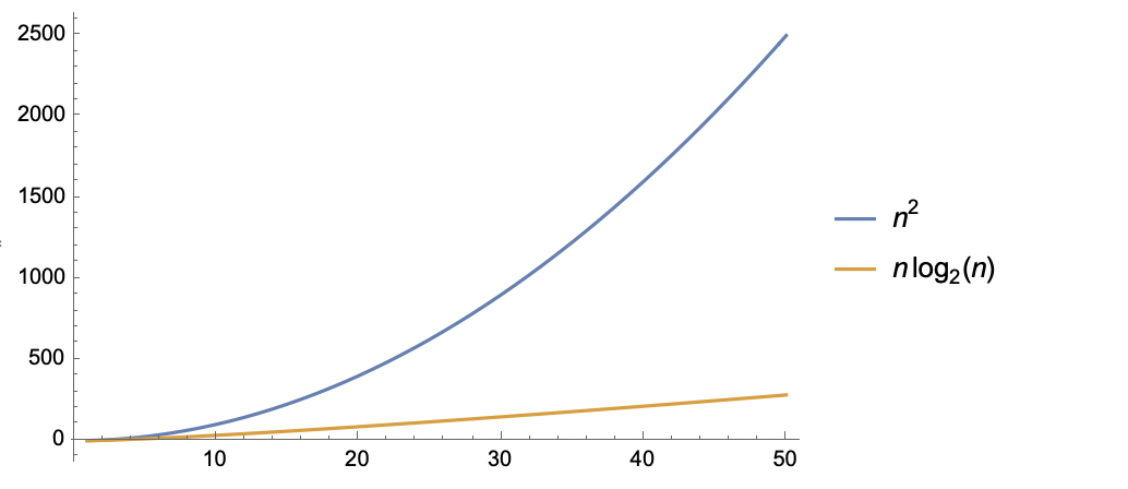
The two sorting algorithms we have seen so far, bubble sort and insertion sort, have worst-case running times of $O(n^2)$. These two algorithms are inefficient as the size of the input array becomes arbitrarily large. This post will introduce two new comparison-based sorting algorithms - merge sort and quick sort, which can run in $O(n\lg n)$ time in all cases (we will use $\lg n$ to denote $log_2\,n$ for this post and all later posts). Asymptotically, this is a tremendous improvement over our previous sorting algorithms. The graph below compares the growth of $f(n)=n^2$ and $f(n)=n\lg n$.

Divide-and-conquer

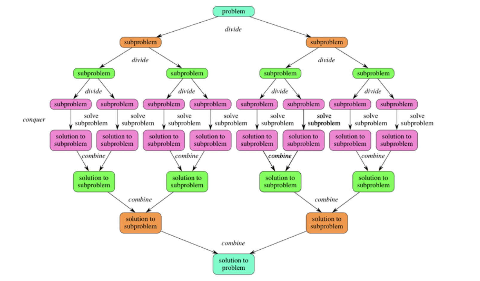
Many useful algorithms employ a common paradigm based on recursion. This paradigm, divide-and-conquer, breaks a problem into several subproblems that are similar to the original problem but smaller in size, recursively solves the subproblems, and finally combine the solutions to the subproblems to create a solution to the original problem.

The divide-and-conquer paradigm involves three steps:

• Divide the problem into a number of subproblems that are smaller instances of the same problem.
• Conquer the subproblems by solving them recursively. If they are small enough, solve the subproblems as base cases.
• Combine the solutions to the subproblems into the solution for the original problem.

Divide-and-conquer process 1

Merge sort

How does merge sort work?

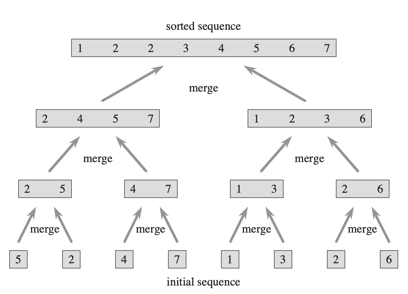
The merge sort employs the divide-and-conquer paradigm. Specifically, it operates as follows

• Divide: Divide the array of $n$ elements into two subarrays of $n/2$ elements each.
• Conquer: Sort the two subarrays recursively using merge sort.
• Combine: Merge the two sorted subarrays.

The algorithm reaches the base case when the subarray has the size of 1, in which there is no work needed to be done because every array of size 1 is already sorted.

The key subroutine of the merge sort algorithm is merging two sorted arrays into a sorted one. We merge by calling an auxiliary function $\text{merge}(A,p,q,r)$, where $A$ is an array and $p,q,$ and $r$ are indices of the array such that $p \le q \lt r$. Assuming that the subarrays $A[p..q]$ and $A[q+1..r]$ are sorted, the $\text{merge}(A,p,q,r)$ function merges them into a single subarray that replaces the current subarray $A[p..r]$.

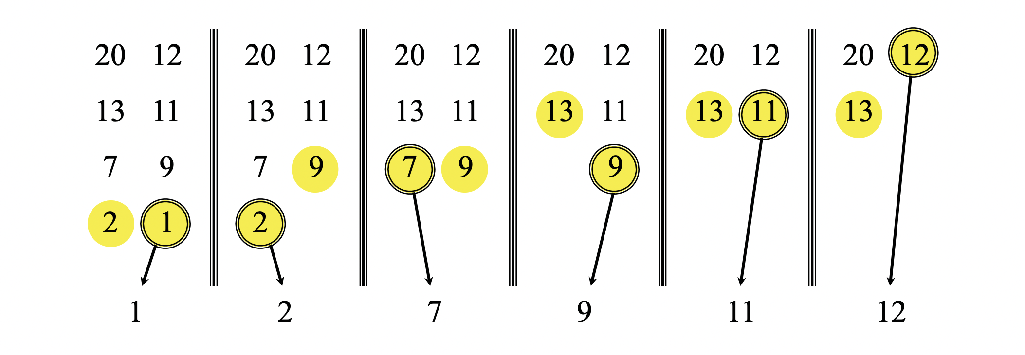
The merging process works as follows:

• First, we have two pointers (indicated by yellow circles) pointing to the smallest elements of two subarrays, which are already sorted.
• We compare the two first elements, then place the smaller element into the output array and move the pointer to the next element of the smaller element. We repeat this step until one input array is empty, at which time we just take the remaining input array and put them into the output array. Comparing two elements takes constant time, and we do it at most $n$ times, where $n=r-p+1$. Therefore, the merge procedure takes $\Theta(n)$.

²

Merge sort implementation

When implementing the merge procedure, we can add a special value $\infty$ to avoid having to check whether each subarray is empty. Whenever the pointer of one subarray moves to $\infty$, all the values of a remaining subarray will be sequentially placed into the output array until this subarray is empty because all values in the remaining subarray are smaller than $\infty$.

def merge(A, p, q, r):
    L, R = [], []
    
    for i in range(p, q + 1):
        L.append(A[i])
    L.append(float('inf'))

    for j in range(q + 1, r + 1):
        R.append[A[j]]
    R.append(float('inf'))

    i = j = 0
    for k in range(p, r + 1):
        if L[i] <= R[j]:
            A[k] = L[i]
            i += 1
        else:
            A[k] = R[j]
            j += 1

We can now use the merge procedure as a subroutine in the merge sort algorithm. The function merge_ sort$(A, p, r)$ sorts the elements in the subarray $A[p..r]$. If $p \lt r$, the algorithm computes an index $q$ that divides $A[p..r]$ into two subarrays: $A[p..q]$, containing $\lceil \frac{n}{2} \rceil$, and $A[q+1..r]$, containing $\lfloor \frac{n}{2} \rfloor$ elements. Otherwise, the subarray has at most one element and is therefore already sorted.

def merge_sort(A, p, r):
    if p < r:
        q = (p + r) // 2
        merge_sort(A, p, q)
        merge_sort(A, q + 1, r)
        merge(A, p, q, r)

Now, we have a complete merge sort program. To sort the array $A = [A[0], A[1], A[n-1]]$, we call merge_sort$(A, 0, n-1)$, where $n$ is the length of the array. The algorithm will recursively partition the initial array into two subarrays until the size of them is 1. Then in the merge procedure, the algorithm involves merging pairs of 1-item arrays to form sorted arrays of length 2, merging pairs of arrays of length 2 to form sorted arrays of length 4, and so forth, until two arrays of length $n/2$ are merged to form the sorted array of length $n$.

³

Complexity analysis

Analysis of divide-and-conquer algorithm

When an algorithm is recursive in its nature, we can analyze the running time of it by using a recurrence equation, which describes the amount of work needed to solve the problem of size $n$ in terms of that needed to solve smaller problems. We can then use mathematics to solve the recurrence for the bounds on the running time of an algorithm.

The recurrence for divide-and-conquer algorithms can be formulated from evaluating three basic steps (divide, conquer, and combine). Let $T(n)$ be the running time on a problem of size $n$. If the problem is small enough, in other words $n \le c$ for some constant $c$, there will be a straightforward solution to the problem, so the running time on it is constant, or we can write as $\Theta(1)$. Suppose that we divide our problem into $x$ subproblems, each of which is $1/y$ the size of the original problem. It takes $T(n/y)$ to solve one problem of size $n/y$, so it takes $xT(n/y)$ to solve $x$ of them. Also, we let $D(n)$ be the time to divide the problem into subproblems and $C(n)$ be the time to combine the solutions to subproblems into the solution to the initial problem. Below is our recurrence for divide-and-conquer algorithms.

\[T(n) = \begin{cases} \Theta(1) & \text{if $n \le c$,} \\ xT(n/y) + D(n) + C(n) & \text{if $n \gt c$.} \end{cases}\]

Analysis of merge sort

To simplify our recurrence analysis, we assume that if $n \gt 1$, then $n$ is always a power of 2, where $n$ is the original problem size. This assumption shall not affect the solution to our recurrence. Knowing that merge sort is a divide-and-conquer algorithm, we start solving the recurrence by analyzing the running time of each part of this paradigm.

Divide: The divide step computes the mid point $q$ of the array, which takes constant time. Hence, $D(n) = \Theta(1)$.

Conquer: We recursively sort two subarrays of $n/2$ elements each, which contributes $2T(n/2)$ to the running time.

Combine: We have already reasoned that merging $n$ elements takes $\Theta(n)$, so $C(n) = \Theta(n)$.

Because the $\Theta(1)$ running time for the divide step is lower-order term when compared to the $\Theta(n)$ running time of the combine step, we can ignore the $\Theta(1)$ part and say that the divide and combine steps together takes $\Theta(n)$ time. (Constant factors will be insignificant as we consider the asymptotic running time). Therefore, we can write our recurrence as follows.

\[T(n) = \begin{cases} \Theta(1) & \text{if $n = 1$,} \\ 2T(n/2) + \Theta(n) & \text{if $n \gt 1$.} \end{cases}\]

To keep things simple, let us rewrite the recurrence as

\[T(n) = \begin{cases} c & \text{if $n = 1$,} \\ 2T(n/2) + cn & \text{if $n \gt 1$.} \end{cases}\]

In the recurrence above, we let the same constant $c$ represent both the time needed to solve the problem of size 1 and the time per element of the divide and combine steps. This does not affect the solution of our recurrence because we use big-$\Theta$ notation, which gives an upper bound and a lower bound on the running time of an algorithm.

Without the master theorem, we can solve this recurrence intuitively by using the recurrence tree.

³

³

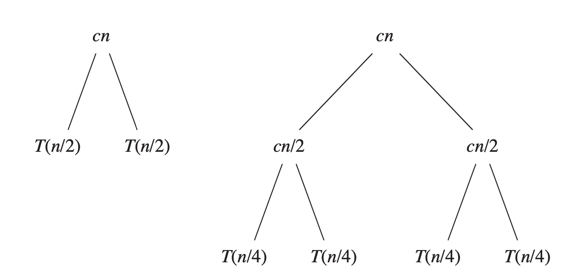
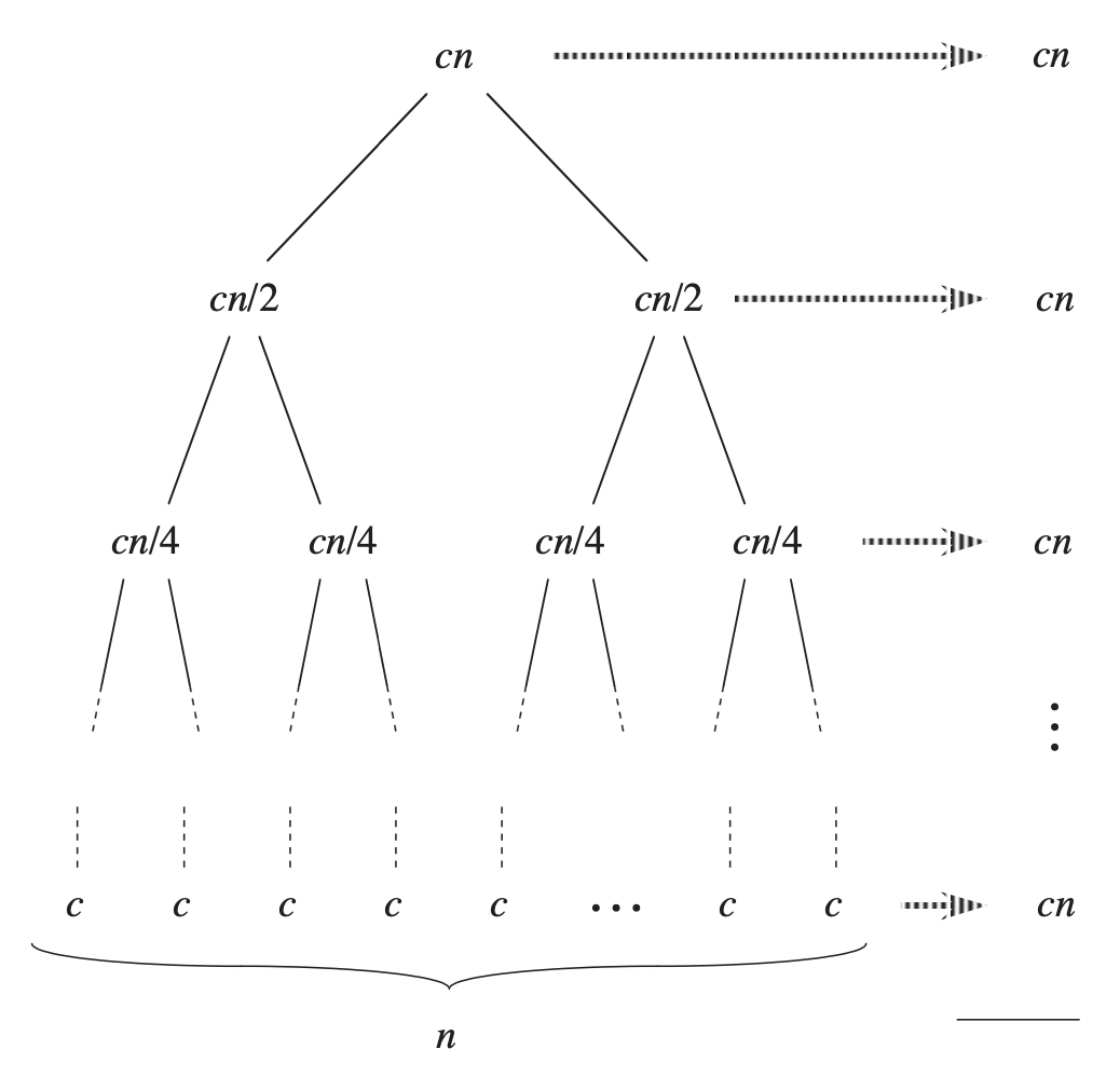
From the images above, we can see that the level $i$ of the tree has $2^i$ nodes (the root is level $0$). Each node representing a subproblem takes $c(n/2^i)$ time to run, so that the cost of level $i$ is $2^i.c(n/2^i)=cn$. Because we start with an array of $n$ elements, there will be $n$ subarrays of size 1. In other words, the last level of the tree has $n$ nodes. To calculate the total running time of the algorithm, we add up the cost of each level, so the merge sort algorithm takes $l.cn$ time to run, where $l$ is the number of levels of the tree.

Now we need to compute $l$ to get the solution. Noting that the bottom level has $n$ nodes, so $2^i = n \iff i = \lg n$. We start at level $0$, so the tree has $\lg n + 1$ levels in total.

Thus, the total cost of the algorithm is $cn(\lg n + 1) = cn\lg n + cn$. When considering the asymptotic running time, we can discard the lower-order term $cn$, giving us the result of $\Theta(n\lg n)$.

In addition, the space complexity for the merge sort algorithm is $O(n)$. Because this algorithm involves recursion, additional memory for “call stack” is required. Although merge sort triggers two recursive calls each time, only one of those two calls executes at a time. The first call on the left part of the array ends before the second call starts. Think about the recursion tree before. This order is equivalent to going to the leftmost branch of the tree until we reach the leaves (bottom) of the recursion tree.

Because the depth of the recursion tree is at most $\lg n + 1$, the maximum height of the “call stack” is $\lg n + 1$.

Moreover, we need to create two subarrays $L$ and $R$ at each level. However, the computer memory will clear those arrays after the function ends. Therefore, we only need at most $O(n)$ auxiliary space when merging two subarrays, each with the size of $n/2$, into the final array.

Hence, the total space complexity for merge sort is $n + \lg n + 1 = O(n)$ (linear factor is dominant over logarithmic factor in terms of asymptotic growth).

Quicksort

Overview

Quicksort is a comparison-based and in-place sorting algorithm developed by British computer scientist Tony Hoare in 1959. It has a worst-case running time of $\Theta(n^2)$ on an input size $n$. However, quicksort is the most widely used sorting algorithm in the real world because it significantly outperforms other algorithms on average. The expected running time of quicksort on the average case is $\Theta(n\lg n)$, and the constant factors hidden in the $\Theta(n\lg n)$ term are quite small. When implemented well, quicksort can be faster than merge sort and around two or three times faster than heapsort.

Working of quicksort algorithm

Like merge sort, quicksort is a divide-and-conquer algorithm. However, the way quicksort applies the divide-and-conquer paradigm is a little different from merge sort. In merge sort, the divide step almost does not do anything, and all the real work happens in the combine step. In contrast, the divide step is the central part of quicksort.

Here is how quicksort employs divide-and-conquer for sorting a subarray $A[p…r]$:

• Divide: Partition the array $A[p…r]$ into two (can be empty) subarrays $A[p…q-1]$ and $A[q+1…r]$ such that all elements in $A[p…q-1]$ are less than or equal to $A[q]$, which must be also less than all elements in $A[q+1…r]$. The $A[q]$ element is often called pivot, and the computation of the index $q$ is key to the partitioning process.

• Conquer: Recursively apply quicksort on two subarrays $A[p..q-1]$ and $A[q+1…r]$.

• Combine: After the partitioning procedure, the pivot element is always at the correct position. Then, we recursively sort two subarrays that do not include the pivot. As a result, the entire array is already sorted, and there is no work to do at this step.

Quicksort algorithm typically follows the below steps:

1. Select the pivot element: There are many ways to select the pivot element: pick the first, the last, the median, or any random element of the array. This section shows how the algorithm works when we choose the last element as a pivot.

2. Partition (rearrange) the array: Suppose we want to partition the array $A[p…r]$. Firstly, we select an element $A[r]$ as a pivot element and initialize variable $i$ with a value of $-1$. This variable will keep track of the index of the last element of the subarray whose all elements are less than or equal to the pivot. Then, we loop through the array $A[p…r]$ from $p$ to $r-1$ using a pointer $j$. If $A[j] \gt A[r]$, we do nothing and keep incrementing $j$. If $A[j] \le A[r]$, we increment $i$ by one and then swap $A[i]$ and $A[j]$. We continue to this process until $j$ reaches $r-1$. Remember that $A[i]$ is the last element in the subarray whose elements are less than or equal to the pivot. Therefore, to put the pivot into its correct position, we swap $A[i+1]$ and $A[r]$. Let $q = i + 1$, we now have a pivot $A[q]$ that is larger than or equal to all elements in $A[p…q-1]$ and strictly less than all elements in $A[q+1…r]$.

3. Recursively sort two subarrays: Recursively call quicksort on $A[p…q-1]$ and then on $A[q+1…r]$.

Because we loop through the subarray $A[p…r]$ once, the running time of partitioning procedure on this subarray is $\Theta(n)$, where $n = r - p + 1$.

Quicksort implementation

def quick_sort(A, p ,r):
    if p < r:
        q = partition(A, p, r)
        quick_sort(A, p, q - 1)
        quick_sort(A, q + 1, r)


def partition(A, p, r):
    pivot = A[r]
    i = p - 1
    for j in range(p, r):
        if A[j] <= pivot:
            i += 1
            A[i], A[j] = A[j], A[i]
    A[i + 1], A[r] = A[r], A[i + 1]
    return i + 1

To sort the entire array $A$, we call quick_sort$(A, 0, len(A) - 1)$.

Randomized quicksort

As we mentioned before, the quicksort algorithm is more efficient than other sorting algorithms on most inputs. However, quicksort performs poorly when the pivot splits the array into extremely unbalanced subarrays (e.g., The size of $A[p…q-1]$ and $A[q+1…r]$ is $0$ and $n-1$, respectively). Therefore, to solve this problem, we can try to add randomization to the algorithm using a technique called random sampling with the hope of getting a good performance on all inputs.

Specifically, instead of always choosing $A[r]$ as the pivot, we can randomly select an element from the subarray $A[p…r]$ as the pivot. Using the random sampling technique, we ensure that each element in the subarray has an equal chance to be the pivot. Doing this way, we can hope that the split of the input array will be well balanced on average.

Randomized quicksort implementation

import random

def randomized_quick_sort(A, p ,r):
    if p < r:
        q = randomized_partition(A, p, r)
        randomized_quick_sort(A, p, q - 1)
        randomized_quick_sort(A, q + 1, r)


def randomized_partition(A, p, r):
    pivot = random.randint(p, r)
    A[pivot], A[r] = A[r], A[pivot]
    return partition(A, p, r)

def partition(A, p, r):
    pivot = A[r]
    i = p - 1
    for j in range(p, r):
        if A[j] <= pivot:
            i += 1
            A[i], A[j] = A[j], A[i]
    A[i + 1], A[r] = A[r], A[i + 1]
    return i + 1

Complexity analysis

The running time of quicksort depends on whether the pivot partitions the array into balanced or unbalanced subarrays. If the partitioning is balanced, the algorithm runs asymptotically as fast as merge sort. However, if the partitioning is unbalanced, the asymptotic running time of quicksort can be as slow as that of insertion sort. In this section, we will investigate the performance of quicksort and the randomized version of it in all cases.

Best-case analysis

The best case happens when the pivot splits the input array into two balanced halves, each with a size no more than $n/2$. In this case, the recurrence for the running time of quicksort is

\[T(n) = 2T(n/2) + \Theta(n)\]

For the sake of simplicity, we can accept that two subproblems have the exact size of $n/2$, and this shall not affect the final result. This recurrence is the same as the recurrence we have solved for merge sort, and its solution is $T(n) = \Theta(n\lg n)$. Therefore, if the pivot partitions the array equally at each level of recursion, the time complexity of quicksort will be $\Theta(n\lg n)$.

Worst-case analysis

Intuitively, we see that the worst case occurs when the partitioning procedure produces one subproblem with $n-1$ elements and one with $0$ elements. Let assume that this worst-case behavior happens in every partitioning routine. The running time of the partitioning is $cn$ for some constant c. The recursive call on the array of size $0$ checks the condition and returns, so this step costs constant time, and we can ignore it when solving the recurrence. The recurrence for the worst-case running time of quicksort is

\[\begin{align} T(n) &= T(n-1) + T(0) + cn \\ &= T(n-1) + cn \\ &= T(n-2) + c(n-1) + cn \\ & \;\;. \\ & \;\;. \\ & \;\;. \\ &= c(n + n - 1 + n - 2 + \ldots + 1) \\ &= \frac{n(n+1)}{2} \\ &= \Theta(n^2) \\ \end{align}\]

The solution to the recurrence above is $T(n) = \Theta(n^2)$, which means that quicksort is not efficient than insertion in the worst case. The running time $\Theta(n^2)$ occurs when the input array is already sorted, while insertion sort has a linear running time.

However, this intuitive result is based on the assumption that at each recursive level, the pivot splits the input array into two maximally unbalanced subarrays. We now will prove this assumption. Let $T(n)$ be the worst-case running time of quicksort on the input of size $n$. We have

\[T(n) = \max_{0 \le q \lt n - 1}(T(q) + T(n - 1 - q)) + \Theta(n)\]

$q$ ranges from $0$ to $n-1$ because the partition function can produce a subproblem of size $0$ up to $n-1$. Also, we guess that $T(n) \le cn^2$. Substituting this inequality into the recurrence above, we get

\[\begin{align} T(n) &\le \max_{0 \le q \lt n - 1}(cq^2 + c(n - 1 - q)^2) + \Theta(n) \\ &= \max_{0 \le q \lt n - 1}(q^2 + (n - 1 - q)^2)\cdot c + \Theta(n) \end{align}\]

The problem here is to find the maximum of function $f(q) = q^2 + (n - 1 - q)^2$ on the interval $[0, n-1]$. Notice that

\[\begin{align} f'(q) &= 2q - 2(n - 1 - q) = 4q -2n + 2 \\ f''(q) &= 4 \end{align}\]

Because $f’' (q) \gt 0, \forall q \in \mathbb{R}$, the graph of this function always concaves up. Therefore, the maximum of $f(q)$ on that interval must occur at either two endpoints $0$ or $n-1$. In this case, both $q=0$ and $q=n-1$ gives us the maximum $(n-1)^2$. Substituting back to our recurrence, we obtain

\[\begin{align} T(n) &\le c(n-1)^2 + \Theta(n) \\ &= cn^2 - c(2n-1) + \Theta(n) \\ &\le cn^2 \end{align}\]

We can pick a large enough constant $c$ so that the $c(2n-1)$ and $\Theta(n)$ term cancel out. Hence, the solution for the recurrence is $T(n) = O(n^2)$. Using a similar method, we can prove that $T(n) = \Omega(n^2)$. Therefore, the worst-case running time of quicksort is $\Theta(n^2)$.

Average-case analysis

The performance of quicksort in the average case is much closer to the best case than to the worst case, meaning that even when the partitioning seems quite unbalanced, quicksort still achieves $O(n\lg n)$ running time. The image below represents the size of subproblems at each level if the partitioning always produces a 9-to-1 split.

³

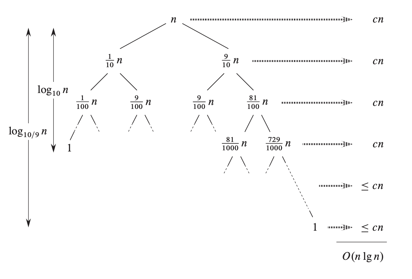
The maximum depth of the recursion tree is $\log_{10/9}n = \Theta(\lg n)$, and the cost at each level is at most $cn$. Thus, quicksort runs in $O(n \lg n)$ time with the split ratio of 9-to-1 at each recursive level. In fact, the time complexity of quicksort is $O(n \lg n)$ when there is a proportional split at each level.

On average, it is extremely unlikely for the partitioning to be always maximally unbalanced on every recursive call. Therefore, we can intuitively say that the expected running time of quicksort is $O(n \lg n)$.

To do a formal analysis on the performance of quicksort, we will analyze the running time of the partitioning function because all the work of quicksort happens in the partitioning step. Each time we call this function, it selects a pivot, and this element is never included in any future procedure. Hence, the partitioning function will run at most $n$ times over the entire execution of the quicksort algorithm. The cost of the partition function depends on the amount of work done in the for loop when we compare the pivot with other elements. Thus, to calculate the total time spent on the partitioning step of the quicksort algorithm, we can count the total number of comparisons in the for loop. Also, we assume that all elements in the input array are distinct.

Let $X$ be the total number of comparisons done in the partitioning procedure of the quicksort algorithm. As we explained before, the running time of quicksort is $O(n + X)$. To make our analysis easier, we rename the elements of the array $A$ as $z_1, z_2,\ldots,z_n$, with $z_i$ being the $i$th smallest element and define the set $Z_{ij} = {z_i, z_{i+1}, \ldots, z_j}$ to be the set of elements between $z_i$ and $z_j$ (inclusive). Also, we define $X_{ij}$ as an event that $z_i$ is compared to $z_j$. Each pair of elements is compared at most once because elements are compared only to the pivot element, and the pivot is never included in any future recursive calls. Therefore, the total number of comparisons performed by the quicksort algorithm is

\[X = \sum_{i=1}^{n-1}\sum_{j=i+1}^{n}X_{ij}\]

Taking the expectation of both sides, we have

\[E(X) = E(\sum_{i=1}^{n-1}\sum_{j=i+1}^{n}X_{ij})\]

Because expectation has the linearity property, the above expression is equivalent to

\[\begin{align} E(X) &= \sum_{i=1}^{n-1}\sum_{j=i+1}^{n}E(X_{ij}) \\ E(X) &= \sum_{i=1}^{n-1}\sum_{j=i+1}^{n}P(\text{$z_i$ is compared to $z_j$}) \tag{1} \end{align}\]

If there is a pivot $x$ such that $z_i \lt x \lt z_j$, $z_i$ and $z_j$ cannot be compared at any time during the quicksort algorithm because the pivot will put $z_i$ and $z_j$ into two separate subarrays. If $z_i$ is selected as a pivot before any other items in $Z_{ij}$, it will be compared to all other elements in $Z_{ij}$ (including $z_j$), except for itself. Hence, $z_i$ and $z_j$ are compared if and only if the first element to be chosen as a pivot from $Z_{ij}$ is either $z_i$ or $z_j$.

Before any element from $Z_{ij}$ is chosen as a pivot, the whole set $Z_{ij}$ is in the same partition. Therefore, each element has the same probability of being first chosen as a pivot. Because the set $Z_{ij}$ has $j - i + 1$ elements, the probability an element is the first one from the set $Z_{ij}$ to be chosen as a pivot is $1/(j - i + 1)$. Also, because the events that $z_i$ is the first pivot from $Z_{ij}$ and that $z_j$ is the first pivot from $Z_{ij}$ are mutually exclusive, we have

\[\begin{align} P(\text{$z_i$ is compared to $z_j$}) &= P(\text{$z_i$ or $z_j$ is first chosen as a pivot}) \\ &= P(\text{$z_i$ is first chosen as a pivot}) \\ &+ P(\text{$z_j$ is first chosen as a pivot}) \\ &= \frac{1}{j - i + 1} + \frac{1}{j - i + 1} \\ &= \frac{2}{j - i + 1} \tag{2} \end{align}\]

Substituting the equation $(2)$ into the equation $(1)$, we obtain

\[\begin{align} E(X) &= \sum_{i=1}^{n-1}\sum_{j=i+1}^{n}\frac{2}{j - i + 1} \\ &= \sum_{i=1}^{n-1}\sum_{k=1}^{n}\frac{2}{k + 1} \\ &\lt \sum_{i=1}^{n-1}\sum_{k=1}^{n}\frac{2}{k} \tag{3} \\ \end{align}\]

Notice that we can calculate $\sum_{k=1}^{n}\frac{2}{k}$ as a Riemann Sum.

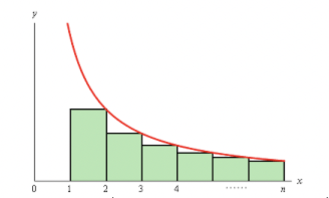
Based on the graph, we have

\[\begin{align} \sum_{k=2}^{n}\frac{1}{k} &\le \int_{1}^{n}\frac{1}{x}\mathrm{d}x \\ &= \ln x \Big|^n_1 \\ &= \ln n \\ \Rightarrow \sum_{k=1}^{n}\frac{2}{k} &\le 2(\ln n + 1) \tag{4} \\ \end{align}\]

Combining $(3)$ and $(4)$, we obtain

\[\begin{align} E(X) &\lt \sum_{i=1}^{n-1}2(\ln n + 1) \\ &= 2(n - 1)(\ln n + 1) \\ &= O(n \lg n) \\ \end{align}\]

Hence, the expected running time of quicksort is $O(n \lg n)$ when all elements of an input array are distinct.

Conclusion

In this post, we have covered two divide-and-conquer sorting algorithms that have an expected running time of $O(n \lg n)$. In future posts, we will introduce other sorting algorithms that use new data structures and find a lower bound for the running time of comparison-based sorting algorithms.

The content of this post is based on the course 6.006 Introduction to Algorithms, Fall 2011 and the book Introduction to Algorithms (CLRS).

References

1. Thomas Cormen, Devin Balkcom, Khan Academy computing curriculum team. Algorithms, Merge sort. CC-BY-NC-SA License ↩

2. Srini Devadas, S. 6.006 Introduction to Algorithms: Lecture 3, Fall 2011. ↩

3. Thomas H. Cormen, Charles E. Leiserson, Ronald L. Rivest, Clifford Stein: Introduction to Algorithms, 3rd Edition. MIT Press 2009, ISBN 978-0-262-03384-8, pp. 30-37 & pp. 170-184. ↩ ↩² ↩³ ↩⁴