Augmented Binary Search Trees, AVL Trees
Introduction
This post will continue from where Runway reservation system and Binary Search Trees left off in designing a binary search tree that supports insertion and deletion in $O(\lg n)$ time. We first investigate how to augment a binary search tree and what information we can get from an augmented binary search tree. Then, we discuss operations to keep the tree balanced, which will allow us to insert or delete an element in $O(\lg n)$ time.
Augmenting data structures
Some engineering situations require no more than a “textbook” data structure, such as a linked list, a binary search tree, and a hash table. However, many others require us to augment a textbook data structure by storing additional information in it. We rarely need to create an entirely new type of data structure. However, augmenting a data structure is not always straightforward because we have to design operations on it in a way such that they maintain the property of that data structure.
Suppose there is a new requirement for the runway reservation system: How many planes are scheduled to land at times $\le t?$. This new requirement necessitates a design amendment - storing the rank of a node in a binary search tree. We define the $i$th rank element in a binary search tree as the node in the tree with $i$th smallest key.
To compute the rank of a node, we will add an attribute $x.size$ to every node $x$ of the binary search tree. This attribute contains the number of nodes in the subtree rooted at $x$ (including $x$ itself), and we call it the size of the subtree. Hence, we have the following formula for calculating the subtree’s size, where the size of node $\text{None}$ is $0$.
\[x.size = x.left.size + x.right.size + 1\]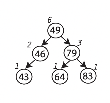 |
|---|
| An augmented binary search tree with node size |
Notice that the size and the rank of a node are different. The size is just a metric we use to compute the rank easier.
Retrieving an element with a given rank
We will begin by looking at an operation that retrieves an element with a given rank. The $\text{select(x, i)}$ returns a pointer to the node containing the $i$th smallest key in the subtree rooted at $x$. To find the $i$th smallest key in an augmented tree $T$, we call $\text{select(T.root, i)}$.
1
2
3
4
5
6
7
8
def select(x, i):
    r = x.left.size + 1
    if i == r:
        return x
    elif i < r:
        return select(x.left, i)
    else:
        return select(x.right, i - r)
Line 2 compute the rank of node $x$ within the subtree rooted a node $x$. Because $x.left.size$ gives the number of nodes that come before $x$ (according to the binary-search-tree property), $x.left.size + 1$ will give the rank of $x$ within the subtree rooted at $x$. If $i = r$, then $x$ is the $i$th smallest element, so we return $x$. If $i < r$, meaning that the $i$th smallest element resides the $x$’s left subtree, we continue to recurse on the left subtree of $x$. If $i > r$, then the $i$th smallest element resides the right subtree. Since there are $r$ elements that come before $x$’s right subtree, the $i$th smallest element in the subtree rooted at $x$ is the $(i - r)$th smallest element in the subtree rooted at $x.right$. Therefore, we call the $\text{select}$ function recursively on $x.right$.
Analysis: Since each recursive call to $\text{select}$ goes down one level of a tree, the worst case running time on a tree of height $h$ is $O(h)$.
Determine the rank of an element
The previous operation gives a sense of working with an augmented data structure. Now, we will design an algorithm that allows us to answer the question: How many landing times $\le t$ are scheduled? This question basically asks us to compute the rank of a node with a key $t$ in a binary search tree.
Given a pointer to node $x$ in an augmented binary search tree $T$, the procedure $\text{rank(T, x)}$ returns the number of elements coming before $x$ (including $x$ itself) in an inorder traversal of $T$.
1
2
3
4
5
6
7
8
def rank(T, x):
    r = x.left.size + 1
    y = x
    while y is not T.root:
        if y is y.parent.right:
            r = r + y.parent.left.size + 1
        y = y.parent
    return r
According to the binary-search-tree property, all elements in $x$’s left subtree are less than $x$, so they will come before $x$ in an inorder tree walk. Line 2 sets $r$ to be the rank of $x$ in the subtree rooted at $x$. We also create a variable $y$ pointing to node $x$ for the sake of argument. If $y$ (also $x$) is the root of the entire tree, we return $r$ as the rank of $x.key$. Otherwise, we continue to go from $x$ upward to the root of the tree. If $y$ is the right child of its parent, all left child of its parent will precede $y$ in the inorder traverse walk. Hence, we add the size of the left subtree of $y$’s parent to $r$. The process ends until we reach the root of the entire tree.
Analysis: In the worst case, we go from the node at the bottom level up to the root, which takes $O(h)$ time, where $h$ is the height of a binary tree.
AVL Tree
Knowing how to augment a data structure, we can now use that idea to design a runway reservation system that supports insertion and deletion in $O(\lg n)$ time. The key problem here is maintaining the binary search tree that stores landing times balanced.
Definition
An AVL tree (named after inventors Adelson-Velsky and Landis) is a binary search tree that balances itself every time an element is inserted or deleted. In addition to the binary-search-tree property, each node of an AVL tree has the property that the heights of subtrees rooted at its left and right child differ at most $1$.
\[|\text{height(node.left)} - \text{height(node.right)}| \le 1\]Upper bound of AVL tree height
We can show that an AVL tree with $n$ nodes has a height of $O(\lg n)$.
Let $N(h)$ denote the minimum number of nodes in an AVL tree of height $h$. Firstly, we see that a tree of height zero has one node, so $N(0) = 1$. Also, a tree of height $1$ contains at least a root and a single root’s child, so $N(1) = 2$.
For $n \ge 2$, let $h_L$ and $h_R$ denote the height of the left and right subtrees, respectively. Because the entire tree has height $h$, one of two subtrees must have height $h-1$, and we suppose that $h_L = h-1$. To minimize the number of nodes, we should make the other subtree as short as possible. By the AVL property, the right subtree must have height $h_R = h-2$. The total number of nodes equals the number of nodes in left and right subtrees plus the root, so we have the following recurrence:
\[\begin{align} N(0) &= 1 \\ N(1) &= 2 \\ N(h) &= N(h-1) + N(h-2) + 1 \\ \end{align}\]Although $N(h)$ is not quite the same as the Fibonacci numbers, by an induction argument, we can show that for large $h$, there is a constant $c$ such that
\[N(h) \ge c\varphi^h \text{, where } \varphi = \frac{1 + \sqrt 5}{2}\]Proof: In addition to the recurrence form, the Fibonacci numbers have the following closed-form
\[F_i = \frac{1}{\sqrt 5}(\phi^i - \hat\phi^i) \tag{*}\]where $\phi$ and $\hat{\phi}$ are the roots of the golden ratio equation $x^2 - x - 1 = 0$:
\[\begin{align} \phi &= \frac{1 + \sqrt 5}{2} \approx 1.618 \\ \hat\phi &= \frac{1 - \sqrt 5}{2} \approx -0.168 \\ \end{align}\]Base case: For $i=0, 1$: $F_0 = 0, F_1 = 1$.
Inductive case: Let $i > 2$ and claim $(*)$ true for all $F_j, j < i$.
\[\begin{align} F_i &\overset{def}= F_{i-1} + F_{i-2} \\ &\overset{(*)}= \frac{1}{\sqrt 5}(\phi^{i-1} - \hat\phi^{i-1}) + \frac{1}{\sqrt 5}(\phi^{i-2} - \hat\phi^{i-2}) \\ &= \frac{1}{\sqrt 5}(\phi^{i-1} + \phi^{i-2}) - \frac{1}{\sqrt 5}(\hat\phi^{i-1} + \hat\phi^{i-2}) \\ &= \frac{1}{\sqrt 5}\phi^{i-2}(\phi + 1) - \frac{1}{\sqrt 5}\hat\phi^{i-2}(\hat\phi + 1) \\ \end{align}\]Since $\phi$ and $\hat\phi$ are solutions to $x^2 - x - 1 = 0 \ \Leftrightarrow x + 1 = x^2$,
\[\begin{align} F_i &= \frac{1}{\sqrt 5}\phi^{i-2}(\phi^2) - \frac{1}{\sqrt 5}\hat\phi^{i-2}(\hat\phi^2) \\ &= \frac{1}{\sqrt 5}(\phi^i - \hat\phi^i) \\ \end{align}\]Because $\lvert \hat\phi \rvert < 1$, we have
\[N(h) = \Theta((\frac{1 + \sqrt 5}{2})^h) \subseteq \Omega(1.618^h)\]and hence
\[\begin{align} N(h) &\ge c\cdot 1.618^h \\ \Rightarrow h &\le 1.44\log_2 n + c' \end{align}\]Therefore, the height of an AVL tree with $n$ nodes is $O(\lg n)$.
Height augmentation
In AVL trees, we augment each node to keep track of the node’s height. We define the height of a node as the longest simple path from the node down to leaves. Below is the Python implementation of node height augmentation.
1
2
3
4
5
6
7
8
def height(node):
    if node is None:
        return -1
    else:
        return node.height

def update_height(node):
    node.height = max(height(node.left), height(node.right)) + 1
Rotation
In order to maintain the tree’s balance, we will employ a simple operation that locally modifies the relationship between two nodes, while preserving the tree’s inorder properties. This operation is call left rotation and right rotation.
 |
|---|
| Right rotation |
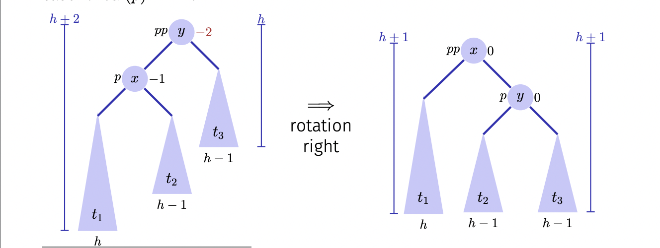
In the image above, the tree at node $y$ is unbalanced because the height of $y$’s left child is $2$ higher than $y$’s right child. Therefore, we need to do a rotation to fix the imbalance. Since the left child $y$ is heavier than its right child, we will perform right rotation on node $y$. Notice that the rotation procedure still maintains the AVL tree property. For example, when doing an inorder traversal on the tree above, we will get $t_1 < x < t_2 < y < t_3$.
1
2
3
4
5
6
7
8
9
10
11
12
13
14
15
16
17
def right_rotate(T, x):
    y = x.left
    y.parent = x.parent
    if y.parent is None:
        T.root = y
    else:
        if y.parent.left is x:
            y.parent.left = y
        elif y.parent.right is x:
            y.parent.right = y
    x.left = y.right
    if x.left is not None:
        x.left.parent = x
    y.right = x
    x.parent = y
    update_height(x)
    update_height(y)
To perform rotation on node $y$ of an AVL tree $T$, we call $\text{right_rotate(T, y)}$.
The left rotation procedure is symmetric the right rotation.
1
2
3
4
5
6
7
8
9
10
11
12
13
14
15
16
17
def left_rotate(T, x):
    y = x.right
    y.parent = x.parent
    if y.parent is None:
        T.root = y
    else:
        if y.parent.left is x:
            y.parent.left = y
        elif y.parent.right is x:
            y.parent.right = y
    x.right = y.left
    if x.right is not None:
        x.right.parent = x
    y.left = x
    x.parent = y
    update_height(x)
    update_height(y)
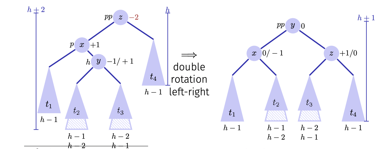
However, in some cases, a single rotation is not sufficient to correct a node that makes the AVL tree unbalanced. In this case, a single rotation does not fix the height of a node that violates the AVL property. Therefore, we need to perform double rotation to solve this problem.
 |
|---|
| Double rotation |
In the example above, to fix the height of node $z$, we call $\text{left_rotate(T, x)}$ and then $\text{right_rotate(T, z)}$. Below is the Python implementation of double rotation.
1
2
3
def left_right_rotate(T, x):
    left_rotate(T, x.left)
    right_rotate(T, x)
AVL insertion
We can insert a node into or delete a node from an AVL tree as we do in a binary search tree. However, after this process, the height invariant of the AVL tree may not be satisfied anymore. As we can see above, after inserting a new node, we have two cases that need to handle. The second case requires at most two rotations, which take $O(1)$ time. Therefore, insertion in an AVL tree takes $O(\lg n)$ time.
AVL deletion
AAVL deletion is not too different from insertion. The key difference here is that unlike insertion, which can only imbalance one node at a time, single deletion of a node may imbalance several of its ancestors. Hence, when we delete a node and cause an imbalance of that node’s parent, not only do we have to make the necessary rotation on the parent, but we have to traverse up the ancestry line, checking the balance, and possibly make some more rotations to fix the AVL tree.
Fixing the AVL tree after a deletion may require making O(log n) more rotations, but since rotations are $O(1)$ operations, the additional rotations do not affect the overall $O(\lg n)$ runtime of a deletion.
AVL rebalance
We will use the $\text{rebalance}$ procedure to maintain the AVL property.
1
2
3
4
5
6
7
8
9
10
11
12
13
14
15
def rebalance(T, node):
    while node is not None:
        if height(node.left) >= 2 + height(node.right):
            if height(node.left.left) >= height(node.left.right):
                left_rotate(T, node)
            else:
                left_rotate(T, node.left)
                right_rotate(T, node.right)
        elif height(node.right) >= 2 + height(node.left):
            if height(node.right.right) >= height(node.right.left):
                left_rotate(T, node)
            else:
                right_rotate(T, node.right)
                left_rotate(T, node)
        node = node.parent
Conclusion
In this post, we finally solve the scheduling problem we discussed before. The key idea here is to maintain the balance of a binary search tree after insertion and deletion. By doing that, we can keep the height of a tree at $O(\lg n)$. Therefore, the running time of operations on that tree will be $O(\lg n)$.
This post is also the last post about sorting and trees topics. In future posts, we will explore graph data structure and graph traversal.