Runway reservation system and Binary Search Trees
Introduction
In this post, we will discuss a real-world problem, which is scheduling times for flights to land on an airport. We often encounter this problem when we want to design a large-scale system that can efficiently handle requests from flights that are going to land. With our current known data structures, we can only solve this problem in $O(n)$ time, where $n$ is the current number of landing times we have scheduled. However, we want to solve this problem in $O(\lg n)$ time, and the new data structure - binary search tree will help us achieve this running time.
Overview
We will first define the scheduling problem by stating our constraints and desired goals. Then, we will elaborate on why current data structures, such as arrays, linked lists, and heaps, cannot do better than linear time. Lastly, we introduce binary search trees and basic operations on the trees. These operations shall help us design a runway reservation system with a running time of $O(\lg n)$.
Runway reservation system
Definition
Given an airport with a very busy single runway, we need to design a runway reservation system for that airport to handle future landing requests. Specifically, each reservation request comes with a landing time of $t$. If there are no other landings within $k$ minutes of requested time $t$, we accept the landing request, meaning that we add $t$ to the set of scheduled landing times. Otherwise, we decline the request and do not add $t$ to our reservation set. When a plane lands safely, we remove its reserved landing time from the scheduling set.
This scenario happens when an airport has multiple runways, but only one runway can be used due to weather conditions, maintenance, etc. In addition, the $k$ minutes check models the case where one plane cannot land right after another because of safety reasons. Therefore, we need to design a system given these constraints.
Example
 |
|---|
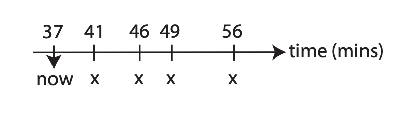
| The timeline of all currently scheduled landings 1 |
Let $R$ denote the set of reserved landing times: $R = \{ 41, 46, 49, 56 \}$ and $k = 3$. If a plane requests for landing at $53$, we accept the request because $53$ is four larger than $49$ and three smaller than $56$. However, if a request comes for landing at $43$, it is declined because it violates the $k$ minutes check. In addition, we do not add a landing time $t$ that is smaller than the minimum of the set $R$ because it is already past.
Our goal is to design a system that can handle requests in $O(\lg n)$ time, where $n$ is the number of elements in the set $R$, or $n = \lvert R \rvert$.
Initial attempts
We can try solving this problem with our current known data structures:
-
Sorted linked list: Appending or prepending a landing time to the list takes constant time, but sorting takes $\Theta(n \lg n)$ time. However, we can insert a new time rather than append or prepend and sort. The $k$ minutes check and insertion take $O(1)$ time because we only need to compare values and change pointers, but finding the insertion point is $\Theta(n)$.
-
Sorted array: It is possible to do a binary search on a sorted array to find the insertion point in $O(\lg n)$ time. Using binary search, we find the smallest index $i$ such that $R[i] \ge t$ - in other words, $R[i]$ is the next larger element of $t$. Then, we compare $R[i-1]$ and $R[i]$ against $t$ and insert $t$ if it passes the $k$ minutes constraint. However, this process takes $\Theta(n)$ because inserting involves shifting elements to the right to make room for a new element.
-
Unsorted list/array: We can add a new landing request to the end of the list/array in $O(1)$ time. However, performing the $k$ minutes check takes $O(n)$ time because we need to scan the entire array/list.
-
Min-heap: Inserting a new item and maintaining the min-heap property takes $O(\lg n)$ time, but checking the constraint takes $O(n)$ time.
-
Dictionary or Python Set: Inserting takes constant time, but the $k$ minutes check takes $\Omega(n)$ time.
Our current known data structures can check the constraint fast but insert slow, or vice-versa. Therefore, we need to devise a new data structure that supports fast check and insertion.
Binary Search Trees (BST)
Definition
A binary search tree, also called an ordered or sorted binary tree, is a rooted binary tree. We can represent a binary search tree by a linked data structure where each node is an object. In addition to a key and satellite data, each node contains attributes left, right, and parent that point to the nodes corresponding to its left child, its right child, and its parent, respectively. If a child or the parent is missing, the respective attribute contains value $\text{None}$. The root node is the only node in the tree whose parent is $\text{None}$.
In a binary search tree, the key of each node must satisfy the binary-search-tree property:
Let $x$ be a node in a binary search tree. For every node $l$ in the left subtree of $x$, then $l.key \le x.key$. For every node $r$ in the right subtree of $x$, then $r.key \ge x.key$.
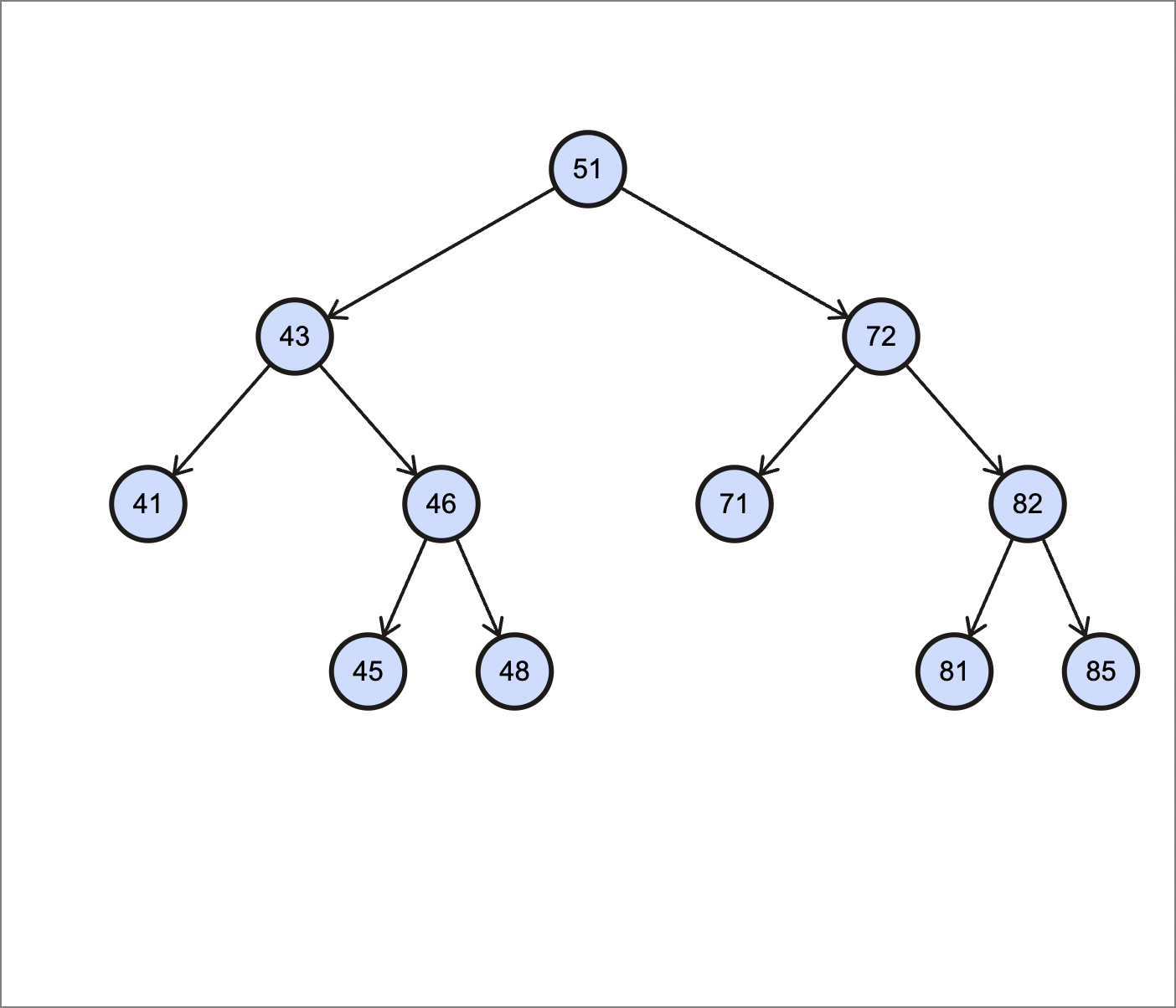 |
|---|
| An example of binary search trees |
As we can see above, the root of our binary search tree has a key of $51$. All the nodes in the left subtree have keys no larger than $51$, and all the nodes in the right subtree have keys no smaller than $51$.
The binary-search-tree property allows us to print out all the keys of a binary search tree in sorted order by using an algorithm called inorder traversal. The algorithm has this name because it prints the root of a subtree between printing the values in its left subtree and printing those in its right subtree. Similarly, a preorder traversal prints the root before the values in either subtree, and a postorder traversal prints the root after the values in both subtrees. Below is the Python implementation of the inorder traversal algorithm. To use this procedure on a binary search tree $T$, we call $\text{inorder_traversal}(T.root)$.
1
2
3
4
5
def inorder_traversal(x):
    if x is not None:
        inorder_traversal(x.left)
        print(x.key)
        inorder_traversal(x.right)
This algorithm goes through all nodes in a binary search tree, so intuitively it takes $\Theta(n)$ time to traverse a binary search tree with $n$ nodes.
Proof. Let $T(n)$ be the time taken by $\text{inorder_traversal}$ when it is called on the root of a $n$-node subtree. Because $\text{inorder_traversal}$ visits all $n$ nodes of the subtree, we have $T(n) = \Omega(n)$. The remaining part of our proof is to show that $T(n) = O(n)$.
If a subtree is empty, the algorithm only needs to do the conditional check x is not None, which takes constant time. Hence, $T(0) = c$ for some constant $c \gt 0$.
For $n \gt 0$, suppose that $\text{inorder_traversal}$ is called on a node $x$ whose left subtree has $k$ nodes and right subtree has $n - k - 1$ nodes. The running time of $\text{inorder_traversal}(x)$ is bounded by $ T(n) \le T(k) + T(n-k-1) + d$, where $d$ is a positive constant that reflects an upper bound on the running time of the body of $\text{inorder_traversal}(x)$, but not including the time complexity of recursive calls inside the body.
We will use the substitution method to show that $T(n) = O(n)$ by proving that $T(n) \le (c+d)n + c$.
- For $n=0$, we have $(c+d)\cdot 0 + c = c = T(0)$
- For $n \gt 0$, we have
Hence, we have $T(n) = \Theta(n)$, meaning that we can go through all the nodes of a binary search tree in linear time. This running time is the same as that of the data structures mentioned at the beginning of the post, which is good news because there is no trade-off here.
Querying a binary search tree
Besides scheduling a landing time, we can also design a runway reservation system that has more information about scheduled landings, such as the most recent scheduled landing time or the least recent landing time. Using a binary search tree, we can support queries: $\text{search}$, $\text{minimum}$, $\text{maximum}$, $\text{successor}$, $\text{predecessor}$. Also, we will examine these operations and discuss how to make each one run in $O(h)$ on any binary search tree of height $h$.
Searching
We use the $\text{search}$ algorithm to search for a node with a key $k$ in a binary search tree. Parameters to this function are a pointer to the root of the tree and a key $k$. The function returns a pointer to a node with a key $k$ if one exists; otherwise, it returns $\text{None}$.
1
2
3
4
5
6
7
def recursive_search(x, k):
    if x is None or k == x.key:
        return x
    elif k < x.key:
        return recursive_search(x.left, k)
    else:
        return recursive_search(x.right, k)
The procedure begins its search at the root and traces a simple path downward in the tree. For each node $x$ it encounters, it compares key $k$ with $x.key$. If the two keys are equal, the search terminates and returns a pointer to node $x$ where $x.key = k$. If $k$ is smaller than $x.key$, the search continues on the left subtree of $x$ because the binary-search-tree property proves that $k$ could not be stored in the right subtree. Symmetrically, if $k$ is larger than $x.key$, the search continues on the right subtree. In the worst case, we go from the root to a leaf of the tree and may or may not find a node with key $k$. Hence, the running time of the searching procedure is $O(h)$, where $h$ is the height of the tree.
This procedure can be implemented iteratively by using a while loop. On most computers, the iterative version is more efficient because computers do not need to allocate additional memory for the call stack.
1
2
3
4
5
6
7
def iterative_search(x, k):
    while x is not None and k != x.key:
        if k < x.key:
            x = x.left
        else:
            x = x.right
    return x
Below is the image of the path that the algorithm goes through to find a key.
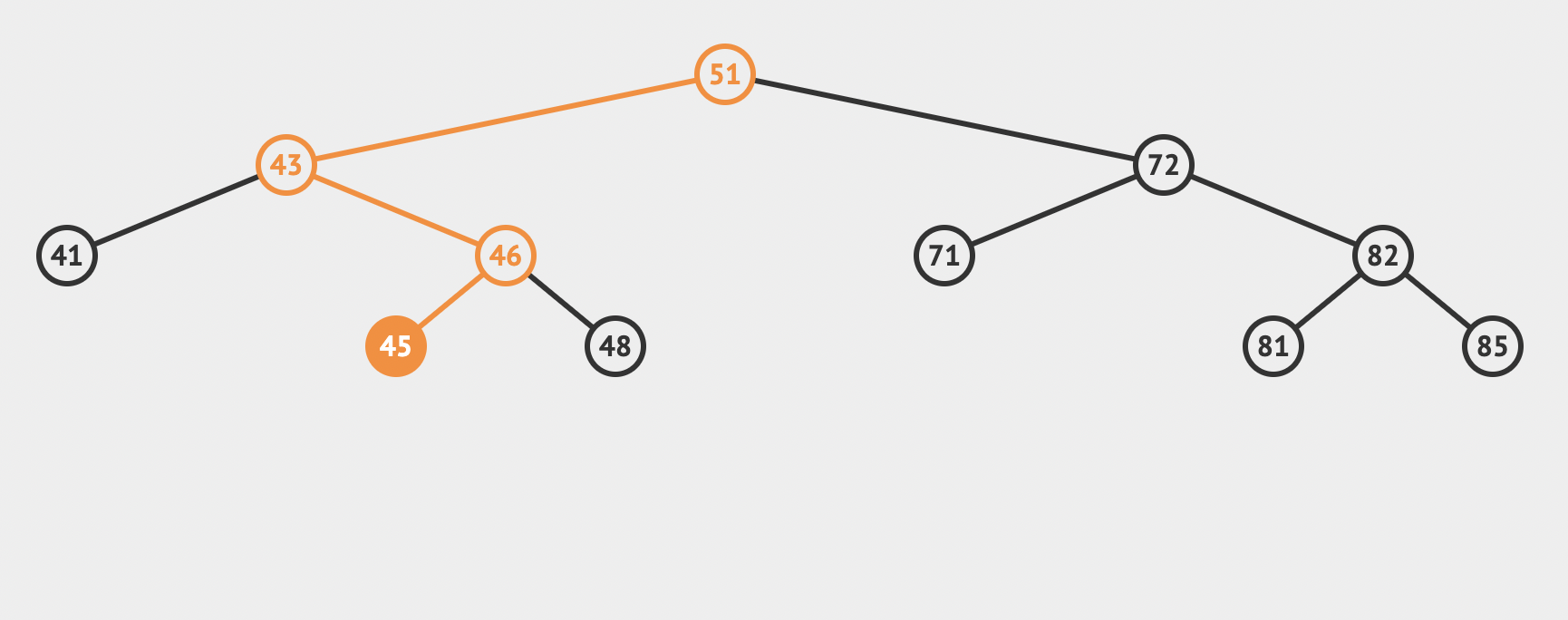 |
|---|
| To search for the key $45$ in the tree, we follow the path $51 \rightarrow 43 \rightarrow 46 \rightarrow 45$ from the root |
Minimum and maximum
To know what is the most recent landing time or the least recent one, we can use the $\text{minimum}$ and $\text{maximum}$ operation on a binary search tree that stores scheduled landing times. To find a minimum key in the tree, we keep following the left subtree from the root until the left subtree is $\text{None}$.
1
2
3
4
def minimum(x):
    while x.left is not None:
        x = x.left
    return x
The binary-search-tree property guarantees that $\text{minimum}$ is correct. If a node $x$ has no left subtree, all nodes in the right subtree of $x$ are not smaller than $x.key$. Hence, the minimum key of the subtree rooted at $x$ is $x.key$. If node $x$ has a left subtree, the node with a minimum key in the subtree rooted at $x$ is the left-most node of the bottom level since no node in the right subtree is not smaller as $x.key$ and every key in the left subtree is not larger than $x.key$.
Symmetrically, we can keep following the right subtree to find a maximum key.
1
2
3
4
def maximum(x):
    while x.right is not None:
        x = x.right
    return x
The running time of these algorithms is $O(h)$ on a tree of height $h$.
Successor and predecessor
Given a scheduled landing time $t$, sometimes we need to find the next landing time (successor), for example, to know if we can accept a new landing time request between these times. If all keys of a binary search tree are distinct, the successor of node $x$ is the node with smallest key greater than $x.key$. We can find the successor of node without comparing keys thanks to the binary-search-tree property.
1
2
3
4
5
6
7
8
def successor(x):
    if x.right is not None:
        return minimum(x.right)
    while x.parent is not None and x is x.parent.right:
        x = x.parent
    return x.parent
To find the successor of node $x$, we have to consider two cases:
-
Case 1: If $x$ has a right subtree where all keys are larger than $x.key$, the next larger key will be the minimum key of the right subtree of $x$.
-
Case 2: If $x$ has no right subtree, we can trace back to ancestor nodes of $x$ until we reach a node that is the left child of its parent. The parent node of that node is the successor of $x$ because the key of that parent node is larger than all keys in its left subtree, including $x.key$.
The procedure to find the predecessor of $x$ is symmetric to $\text{successor}$.
1
2
3
4
5
6
def predecessor(x):
    if x.left is not None:
        return maximum(x.left)
    while x.parent is not None and x is x.parent.left:
        x = x.parent
    return x.parent
In the worst case, the $\text{successor}$ or $\text{predecessor}$ procedure needs to traverse through the longest branch of the tree. Therefore, the running time of these algorithms on a tree of height $h$ is $O(h)$.
Insertion and deletion
We now come to the main part of our runway reservation system, which is to design an algorithm that allows inserting or deleting a landing time in $O(\lg n)$ time. Because we keep the set of scheduled landing times as a binary search tree, insertion and deletion operations on that set must maintain the binary-search-tree property. As we will see later, inserting a new element into the tree is straightforward, but handling deletion is somewhat intricate.
Insertion
Below is the Python code of the $\text{insert}$ procedure for inserting a new value $v$ into a binary search tree. This function takes in a binary search tree $T$ and a new node $z$ where $z.key = v$, $z.left = \text{None}$, and $z.right = \text{None}$.
1
2
3
4
5
6
7
8
9
10
11
12
13
14
15
16
def insert(T, z):
    x = T.root
    y = None                #Keep parent node
    while x is not None:
        y = x
        if z.key < x.key:
            x = x.left
        else:
            x = x.right
    z.parent = y
    if y is None:
        self.root = z       #Tree is empty
    elif z.key < y.key:
        y.left = z
    else:
        y.right = z
The $\text{insert}$ procedure begins at the root of the tree and traces a simple path downward using the pointer $x$ until it reaches $\text{None}$, meaning that we find the available position to insert node $z$. The algorithm uses $y$ as a pointer to the parent of $x$ because by the time we find the place to insert $z$, we go one step over the parent node of $z$. Hence, we cannot update the child pointer of the parent node or parent pointer of node $z$ without keeping the $y$ pointer.
In addition, we can do the $k$ minutes check during insertion. If we find a node with a key within $k$ of new value $v$, we terminate the $\text{insert}$ procedure.
In the worst case, we have to go through the longest path to find available positions for insertion. Hence, the running time of $\text{insert}$ on a tree height $h$ is $O(h)$.
Deletion
When a plane lands safely, we can remove its reserved landing time from the scheduling set using the $\text{delete}$ procedure. The overall method for deleting a node $z$ from a binary search tree $T$ has three cases:
-
Case 1: If $z$ has no children, we simply remove it by changing the child pointer of $z$’s parent to $\text{None}$.
-
Case 2: If $z$ has only one child, we replace $z$ with that child by modifying $z$’s parent to have $z$’s child as its child.
-
Case 3: If $z$ has two children, we will find $z$’s successor $y$, which must be in the right subtree of $z$, and we have $y$ take the position of $z$. This case is quite complicated because it depends on whether $y$ is $z$’s right child.
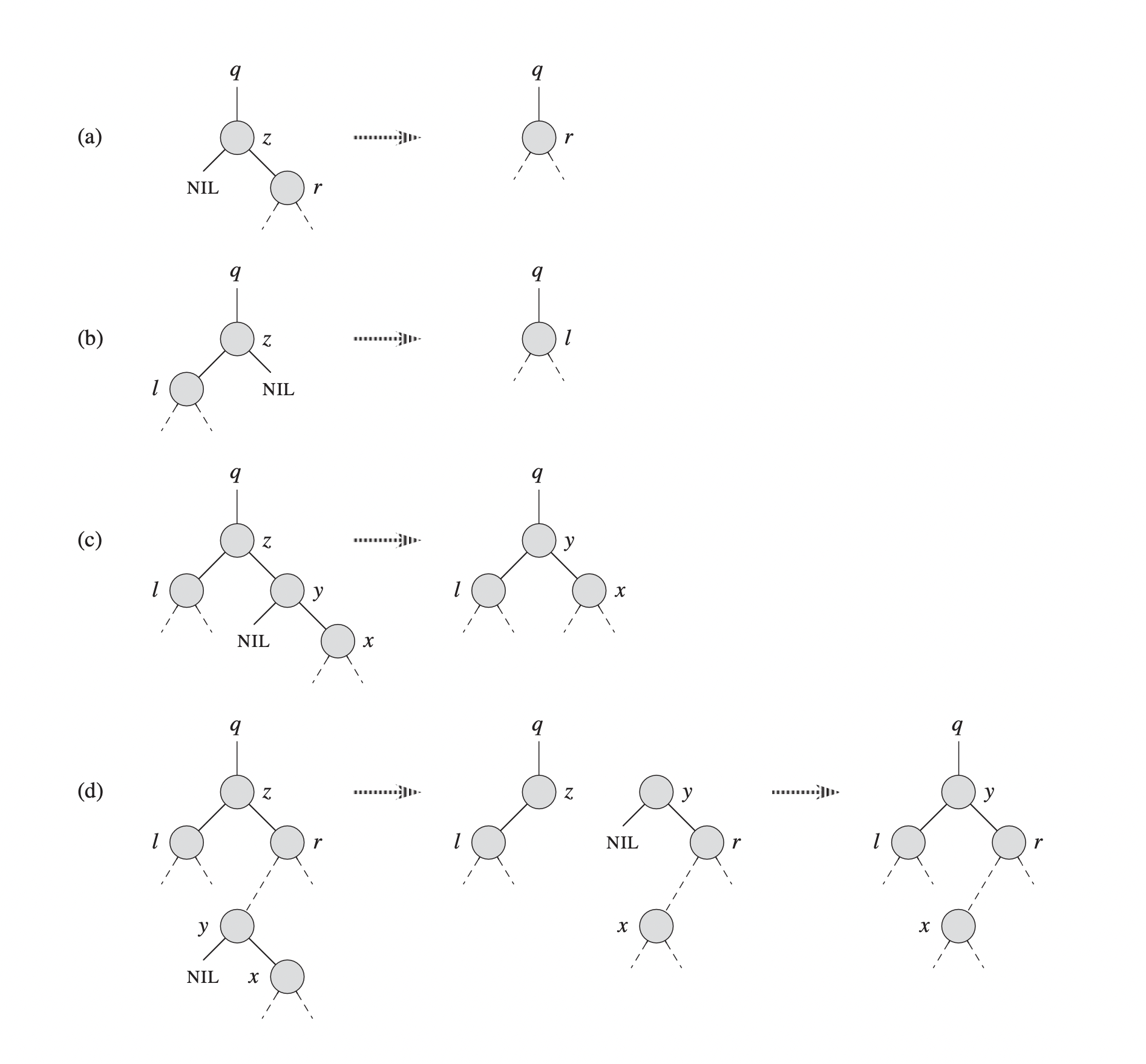 |
|---|
| Example of deleting a node $z$ from a binary search tree |
The function for deleting a node $z$ from a binary search tree $T$ takes pointers to $T$ and $z$ as parameters. It follows three cases we specified above:
-
If $z$ has only a left child or only a right child, we replace $z$ with its child (case 2). Because $z$’s child can be $\text{None}$, we also cover the first case, which is $z$ has no children.
-
If $z$ has both left and right child, we find $z$’s successor $y$, which must be in the right subtree of $z$ and have no left child. There are two sub-cases in this case:
- If $y$ is $z$’s right child (part (c)), we replace $z$ with $y$ by changing the left child pointer of $y$ from $\text{None}$ to $z$’s left child and leaving $y$’s children untouched.
- If $y$ is not $z$’s right child (part(d)), we first let $y$’s right child take $y$’s position, and then we replace $z$ with $y$.
In order to move subtrees around within the binary search tree, we define a subroutine $\text{transplant}$, which replaces one subtree with another subtree. When $\text{transplant}$ replaces a subtree rooted at node $u$ with another subtree rooted at node $v$, $u$’s parent become $v$’s parent, and $u$’s parent has $v$ as its new child.
1
2
3
4
5
6
7
8
9
def transplant(T, u, v):
    if u.parent is None:
        T.root = v
    elif u is u.parent.left:
        u.parent.left = v
    else:
        u.parent.right = v
    if v is not None:
        v.parent = u.parent
Line 2-3 handle the case where $u$ is the root of $T$. Line 4-5 update $v$ as a left child of $u$’s parent if $u$ is a left child. Line 6-7 perform a similar process if $u$ is a right child. Node $v$ can be $\text{None}$, and if $v$ is not $\text{None}$, we update $v.parent$. Notice that the $\text{transplant}$ algorithm does not update $v.left$ or $v.right$, so we have to do it separately if necessary.
Using the $\text{transplant}$ algorithm, we can delete a node $z$ from a binary search tree $T$ as below.
1
2
3
4
5
6
7
8
9
10
11
12
13
14
def delete(T, z):
    if z.left is None:
        transplant(T, z, z.right)
    elif z.right is None:
        transplant(T, z, z.left)
    else:
        y = minimum(z.right)
        if y.parent is not z:
            transplant(T, y, y.right)
            y.right = z.right
            y.right.parent = y
        transplant(T, z, y)
        y.left = z.left
        y.left.parent = y
Lines 2-5 handle the case where $z$ has only one child. Lines 6-14 deal with the case where $z$ has two children. Because $z$ has a non-empty right subtree, its successor must be the node in that subtree with the smallest key. If $y$ is not $z$’s right child, we will replace $y$ as a child of its parent with $y$’s right child (line 9). Then, lines 10-11 update $z$’s right child to be $y$’s right child. Lines 12-14 replace $z$ as a child of its parent with $y$ and turn $y$’s left child from $\text{None}$ to be $z$’s left child.
Each line of $\text{delete}$ takes constant time, including calls to $\text{transplant}$, but the call to $\text{minimum}$ takes $O(h)$ time. Hence, the total running time of $\text{delete}$ on a tree height $h$ is $O(h)$.
Have we solved the problem?
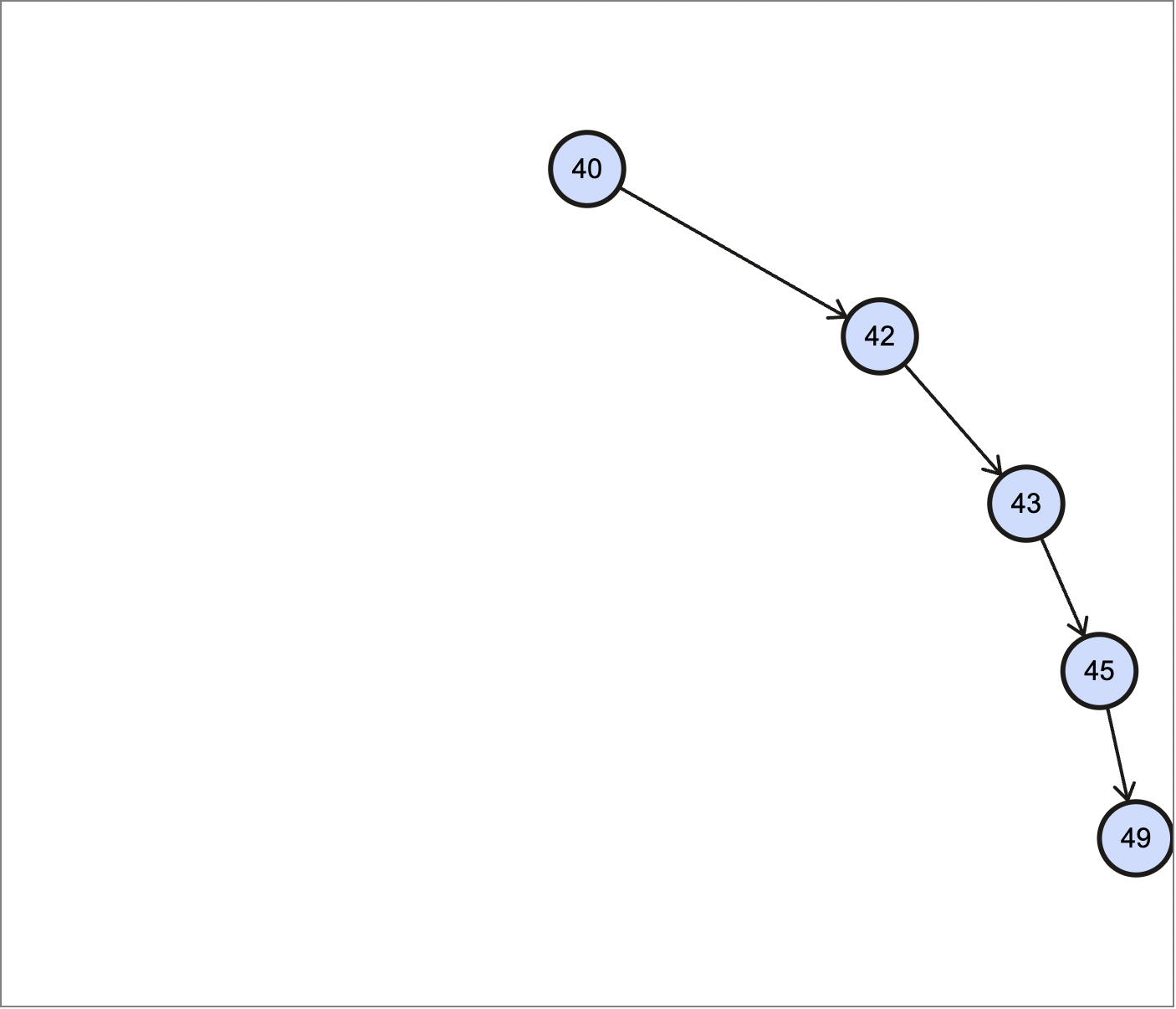
Our goal is to design a runway reservation system that supports insertion and deletion in $O(\lg n)$ time, where $n$ is the number of scheduled landing times. However, up to now, we can only do insertion or deletion on a binary search tree of height $h$ in $O(h)$ time. Therefore, to achieve the $O(\lg n)$ running time, the height of our binary search tree must be $O(\lg n)$, where $n$ is the number of nodes. However, this is not always the case. Consider the following tree.
 |
|---|
| Left-skewed binary search tree |
The binary search tree above has $5$ nodes, and the height of it is exactly equal to the number of nodes. In general, if a binary search tree is extremely skewed, the height of it is $O(n)$, where $n$ is the number of nodes. Hence, querying, insertion, and deletion operations on this tree will take $O(n)$ time, which is not our desired result.
To get the logarithmic running time, we have to keep the binary search tree balanced, and we will investigate how to keep the tree balanced in the future post.
Conclusion
In this post, we defined the runway reservation problem and showed how arrays, linked lists, and hash tables cannot support insertion and deletion in $O(\lg n)$ time. Then, we defined the binary-search-tree property and illustrated basic operations on a binary search tree. The running time of these operations depends on the height of the binary search tree, which is not always $O(\lg n)$. Therefore, we have not solved the problem yet. In the next post, we will see how to keep a binary search tree balanced after inserting or deleting a node of it. A balanced tree shall give us the answer to the scheduling problem.
References
-
Srini Devadas, S. 6.006 Introduction to Algorithms: Lecture 3, Fall 2011. ↩